POLS0010: Data Analysis 2024

Week 6 Task Solution

Here is a worked example of how to produce a series of maps that show the distribution of crime for London.

To make our lives easier we can focus on Camden:

Do particular crime types appear to cluster together?
Are they related to demographic data?

First download the crime data from the data.police.uk website. In this case we are going to tick the “Metropolitan Police” box and then “July” in both the date range dropdowns to get one month of data. Unzip the CSV and place it in a convenient directory.

Now load in packages we need, set the working directory and load in the data. All the steps can be repeated for the December data too.

library(rgdal) # remember tick box may be better
library(sf)

police_data<- read.csv("worksheet_data/2023-07-metropolitan-street.csv")

The next step is to extract only those crimes occurring in Camden. We can us the grepl function for this. This will scan down the rows of a column we specify and extract those that contain a particular word or phrase. In our case we’re looking for Camden so the code is grepl('Camden', police_data$LSOA.name). If you run this on its own you will get a vector that contains TRUE or FALSE to indicate each row with the word. We can combine this step with the usual [ ] to select only the rows that are returned TRUE.

police_data<- police_data[grepl('Camden', police_data$LSOA.name),]

Note how police_data has fewer rows in it. If you type head(police_data) you should see only Camden is present. You should also see a number of columns and recognise what some of them are for.

head(police_data)

##       Crime.ID   Month                 Reported.by                Falls.within
## 13372          2023-07 Metropolitan Police Service Metropolitan Police Service
## 13373          2023-07 Metropolitan Police Service Metropolitan Police Service
## 13374          2023-07 Metropolitan Police Service Metropolitan Police Service
## 13375          2023-07 Metropolitan Police Service Metropolitan Police Service
## 13376          2023-07 Metropolitan Police Service Metropolitan Police Service
## 13377          2023-07 Metropolitan Police Service Metropolitan Police Service
##       Longitude Latitude                    Location LSOA.code   LSOA.name
## 13372 -0.142534 51.56451    On or near Raydon Street E01000907 Camden 001A
## 13373 -0.142623 51.56410   On or near Balmore Street E01000907 Camden 001A
## 13374 -0.142478 51.56305 On or near Winscombe Street E01000907 Camden 001A
## 13375 -0.142623 51.56410   On or near Balmore Street E01000907 Camden 001A
## 13376 -0.142534 51.56451    On or near Raydon Street E01000907 Camden 001A
## 13377 -0.142534 51.56451    On or near Raydon Street E01000907 Camden 001A
##                  Crime.type Last.outcome.category Context
## 13372 Anti-social behaviour                            NA
## 13373 Anti-social behaviour                            NA
## 13374 Anti-social behaviour                            NA
## 13375 Anti-social behaviour                            NA
## 13376 Anti-social behaviour                            NA
## 13377 Anti-social behaviour                            NA

Our priority here are the latitude and longitude columns in order that we can create a dot map. It is worth noticing, however, that some locations have had more than one crime occur. If we did a plot of these they would appear on top of one another so its better to aggregate these to create a data frame that has the number of crimes of each type by location. To do this we need to use the aggregate() function on the Longitude, Latitude, LSOA.code (this will be useful later), and Crime.type columns.

#By using FUN=length we are asking that the aggregate function counts the number of times a crime.ID appears at a location.
crime_count<- aggregate(police_data$Crime.ID, by=list(police_data$Longitude, police_data$Latitude,police_data$LSOA.code,police_data$Crime.type), FUN=length)

#We need to rename our columns (note these are abbreviated from the originals)
names(crime_count)<- c("Long","Lat","LSOA","Crime","Count")

Now we are ready to convert this to spatial data object in R by specifying that the Long/Lat columns (columns 1 & 2) contain this information. Note that we specify EPSG: 4326 as our projection system.

crime_count_sf<-st_as_sf(x = crime_count,                         
           coords = c("Long", "Lat"),
           crs = "+init=epsg:4326")

plot(crime_count_sf)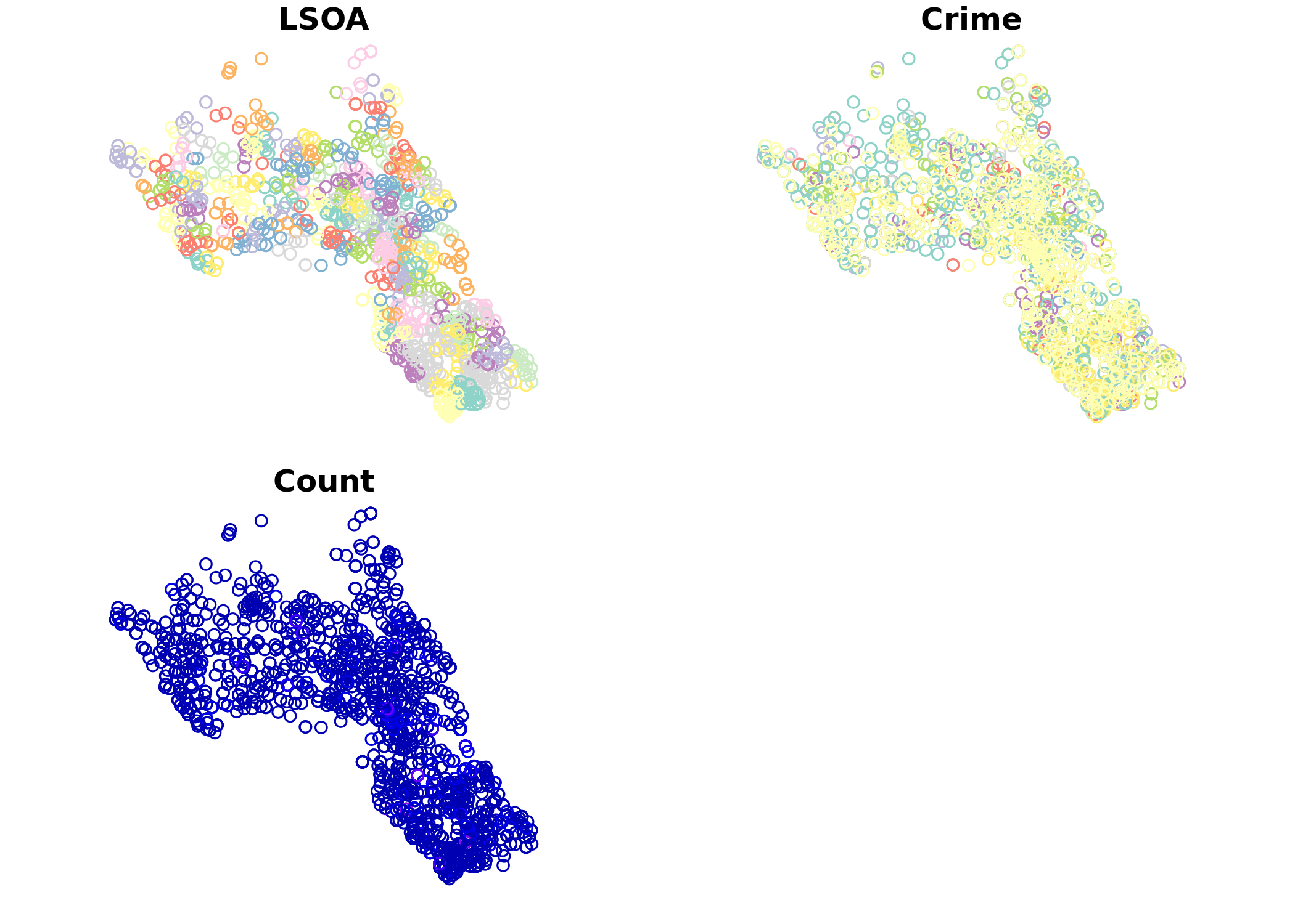

We’re now ready to produce a simple map using tmap. To add the additional layers such as the LSOA boundaries and demographic data revisit the “Mapping Point Data in R” worksheet. In the code below both the size of the bubble represents the count of the crimes and its colour is determined by type of crime that occurred.

tm_shape(crime_count_sf) + tm_bubbles(size = "Count", col = "Crime", legend.size.show = FALSE) +
  tm_layout(legend.text.size = 1.1, legend.title.size = 1.4, frame = FALSE)

You can adjust some of the colour parameters etc to make this map look a little clearer. However, you will notice that there is a lot of overplotting as different crime types in the same location are plotted one on top of another. tmap has a clever function called tm_facets that will create one map for each crime type for us.

tm_shape(crime_count_sf) + tm_bubbles(size = "Count", legend.size.show = FALSE) +
  tm_layout(legend.text.size = 1.1, legend.title.size = 1.4, frame = FALSE)+tm_facets(by="Crime")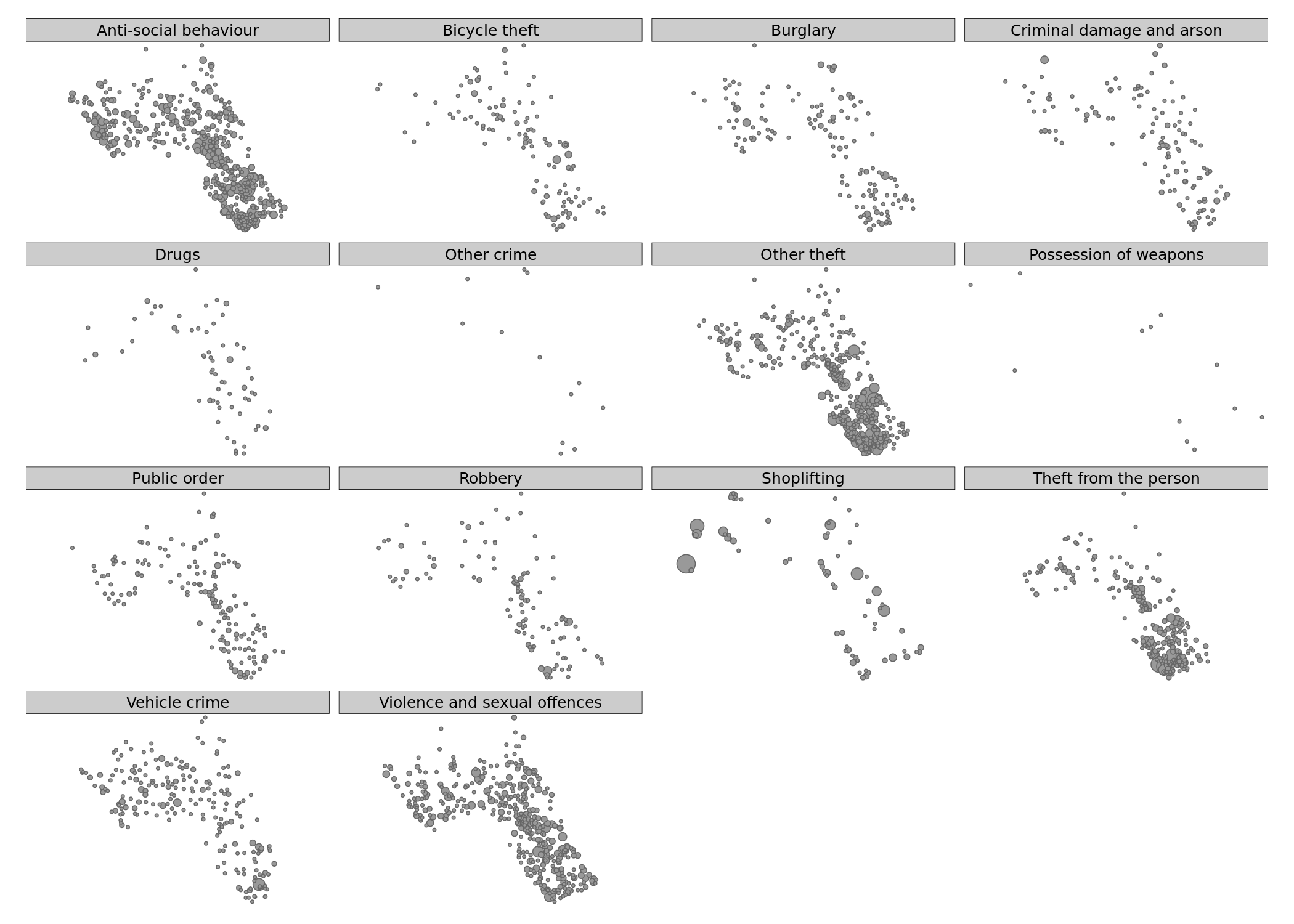

We can then make this a bit clearer with some transparency on the circles using the alpha= parameter.

 tm_shape(crime_count_sf) + tm_bubbles(size = "Count", legend.size.show = FALSE, alpha=0.5) +
  tm_layout(legend.text.size = 1.1, legend.title.size = 1.4, frame = FALSE)+tm_facets(by="Crime")

There’s a lot you can do to build up these plots further – so play around with the different options.

Advanced Solution: Aggregating to Polygon Data

Another way to investigate crimes in Camden would be to count the number of crimes in each LSOA polygon and map it as a choropleth. I would not have expected you to do this for the extension task, but it is a nice advanced step that I will explain more in class.

At the moment we have our data organised with the crime types as separate rows. So each LSOA will have multiple rows – one per count of crime type. We can’t join these rows to our spatial data object, we need one row per LSOA to match it. Therefore we should create a table with columns for each crime type and a single row per LSOA. In technical terms we need to go from a long format to a wide format for the data. For this we go back to the police_data object (before it was converted to a spatial format) and we use the spread function to create the format we need. You first need to install the tidyr package and then load it.

library(`tidyr`)

#Reload in the police data
police_data<-read.csv("worksheet_data/2023-07-metropolitan-street.csv")

#First aggregate the data to each LSOA (rather than the specific latitude and longitude as we did before)

crime_LSOA<- aggregate(police_data$Crime.ID, by=list(police_data$LSOA.code,police_data$Crime.type), FUN=length)

#We need to rename our columns (note these are abbreviated from the originals)
names(crime_LSOA)<- c("LSOA","Crime","Count")

# The arguments to spread():
# - data: Data object
# - key: Name of column containing the new column names
# - value: Name of column containing values

crime_LSOA<- spread(crime_LSOA,Crime, Count)

If you look at the data frame we’ve just created it is is now possible to see we have columns for each crime type and their counts (NAs mean there was no reported crime). Now we can join to our spatial object.

So we need to load this in. You will find the required file in the data folder, see code block below for file name etc. This file has come from the Office for National Statistics’ Geoportal, which contains all manner of geographic data files.

LSOA<- st_read("worksheet_data/Lower_layer_Super_Output_Areas_2021_EW_BGC_V3.geojson")

## Reading layer `Lower_layer_Super_Output_Areas_2021_EW_BGC_V3' from data source `/nfs/cfs/home3/ucfa/ucfa012/POLS0010_2023/worksheet_data/Lower_layer_Super_Output_Areas_2021_EW_BGC_V3.geojson' using driver `GeoJSON'
## Simple feature collection with 35672 features and 8 fields
## geometry type:  MULTIPOLYGON
## dimension:      XY
## bbox:           xmin: 82668.52 ymin: 5352.6 xmax: 655653.8 ymax: 657539.4
## projected CRS:  OSGB 1936 / British National Grid

If we look at the head() of the LSOA object we can see what field in its data frame we can use to join the crime object to.

head(LSOA@data)

In this case there are a number of columns but – as luck would have it – there is a LSOA21CD column which is just what we need!

BUT, remember this is a national file, so just as we did with the OA file in the census data practical we need to take out only those LSOAs that correspond to Camden.

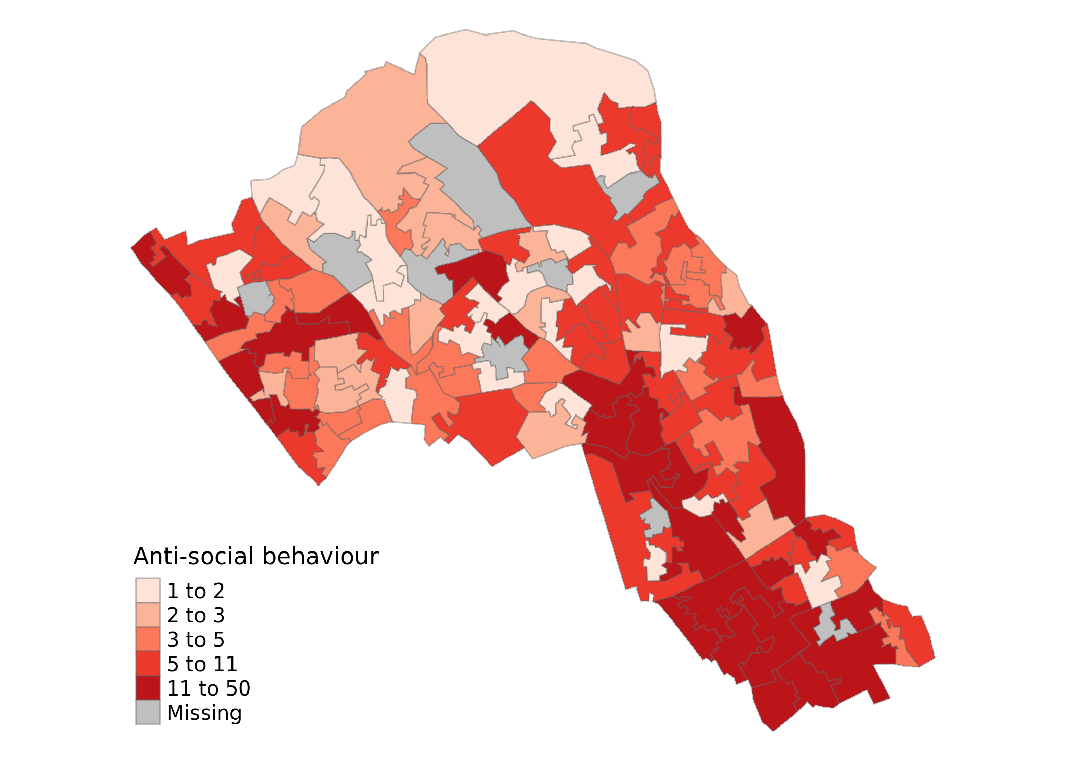
LSOA.Camden<- LSOA[grepl('Camden', LSOA$LSOA21NM),]

LSOA_crime_sf<- merge(LSOA.Camden, crime_LSOA, by.x="LSOA21CD", by.y="LSOA")

Phew! Almost there! We’ve now got our spatial object with the counts per crime that are ready for mapping. Here we map the counts of Anti-social behaviour in the borough.

tm_shape(LSOA_crime_sf) + 
  tm_fill("Anti-social behaviour", palette = "Reds", style = "quantile", title = "Anti-social behaviour") +
  tm_borders(alpha=.4) + tm_layout(legend.text.size = 0.8, legend.title.size = 1.1, frame = FALSE)

James Cheshire

Week 6 Task Solution

Advanced Solution: Aggregating to Polygon Data

Spotlight