Week 9 Solution: Point Pattern Analysis
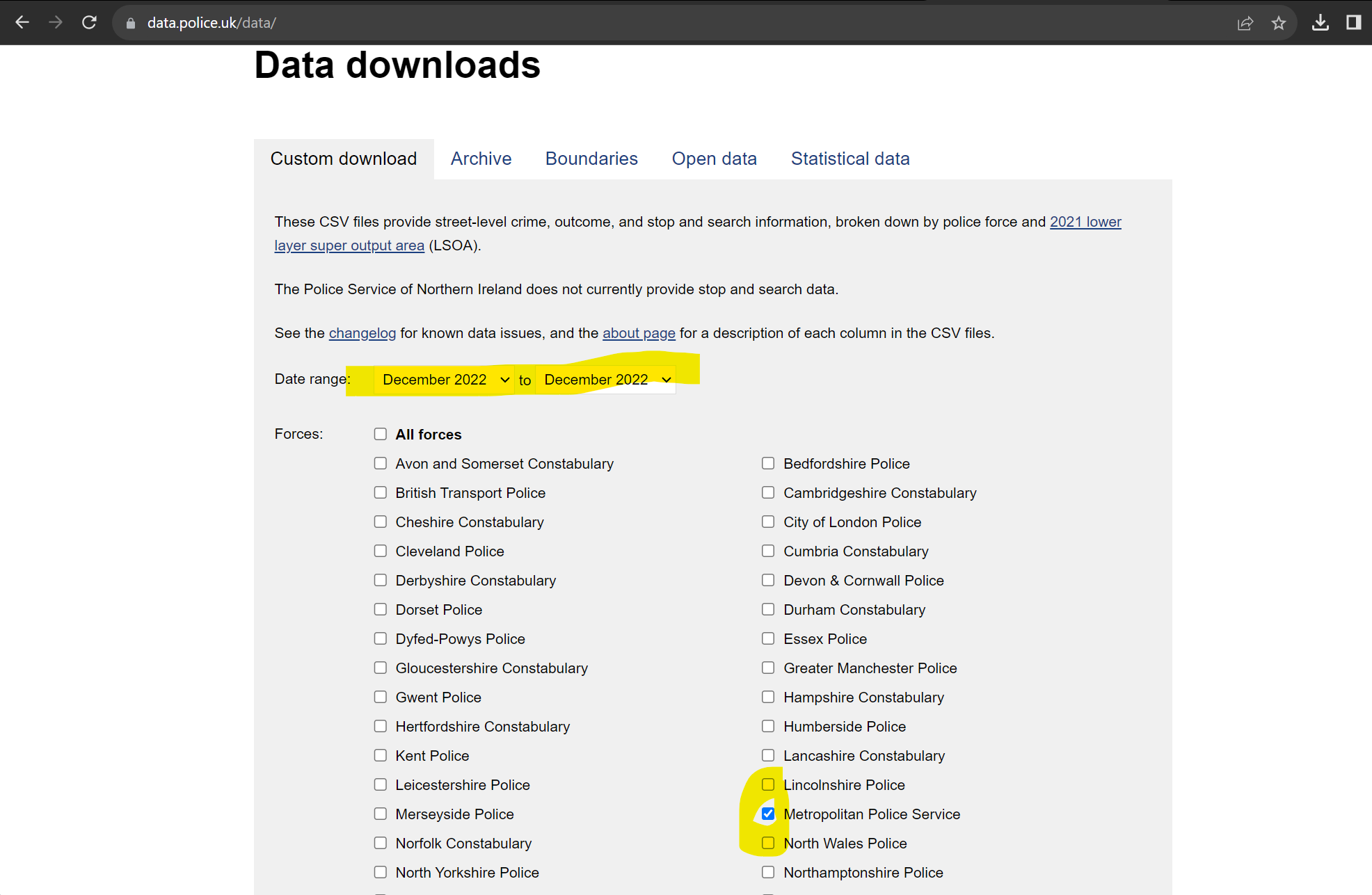
Task 1: Create a DBSCAN crime map of anti-social behaviour for the London Borough of Kensington and Chelsea in December 2022. Data can be downloaded from the data.police.uk website.
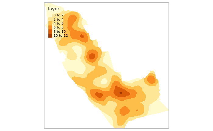
Task 2: Create a crime hotspot map (using KDE) of anti-social behaviour for the London Borough of Kensington and Chelsea in December 2022.
library(sf)
library(spatstat)
library(tmap)
library(dbscan)
setwd("~/POLS0010_2023")

london <- st_read("worksheet_data/london_boroughs.geojson")

kens<- london[grepl('Kensington', london$NAME),]
st_crs(kens) <- 27700

police_data<- read.csv("worksheet_data/2022-12-metropolitan-street.csv")

police_data<- police_data[grepl('Kensington', police_data$LSOA.name),]

#By using FUN=length we are asking that the aggregate function counts the number of times a crime.ID appears at a location.
crime_count_raw<- aggregate(police_data$Crime.ID, by=list(police_data$Longitude, police_data$Latitude,police_data$LSOA.code,police_data$Crime.type), FUN=length)

#We need to rename our columns (note these are abbreviated from the originals)
names(crime_count_raw)<- c("Long","Lat","LSOA","Crime","Count")

#Subset to antisocial behaviour

crime_count_asb<- crime_count_raw[which(crime_count_raw$Crime=="Anti-social behaviour"),]

crime_count_sf<-st_as_sf(x = crime_count_asb,
           coords = c("Long", "Lat"),
           crs = "+init=epsg:4326")

# reproject to British National Grid
crime_count_sf<- st_transform(crime_count_sf, 27700)


plot(crime_count_sf)

#first extract the coordinates from the spatial points data frame
Crime.Points.coords <- st_coordinates(crime_count_sf)

#now run the dbscan analysis
db <- dbscan(Crime.Points.coords, eps = 100, MinPts = 4)
#now plot the results
plot(Crime.Points.coords, col=factor(db$cluster), main = "DBSCAN Output", frame = F, asp=T)

plot(kens, add=T)

#Task 1 completed!

# now onto task 2


library(SpatialKDE)

raster <- create_raster(crime_count_sf, cell_size = 25)

kde_estimate_raster <- kde(crime_count_sf, band_width = 500, grid = raster)


tm_shape(kde_estimate_raster)+tm_raster()

# mask the raster by the output area polygon
masked_kde <- raster::mask(kde_estimate_raster, kens)

# maps the masked raster, also maps white output area boundaries
tm_shape(masked_kde) + tm_raster()