Week 8: Geographically Weighted Regression (GWR)
In this session we will:
- Run a linear model to predict the occurrence of a variable across small areas.
- Run a geographically weighted regression to understand how models may vary across space.
- Print multiple maps in one graphic using gridExtra() with tmap.
Slides for this week can be downloaded here.
First, ensure that your working directory is set to the correct folder and then we can load in the “Census_OA_Shapefile.geojson”.
# load the spatial libraries
library("sf")
library("tmap")

# Remember to set the working directory as usual

OA.Census<-st_read(dsn = "worksheet_data/Census_OA_Shapefile.geojson")
Run a linear model
Before we tackle the ‘geographical’ component of GWR we should first do a basic regression to understand the global relationship across our study area. In this case, the percentage of people with qualifications is our dependent variable, and the percentage of unemployed economically active adults and White British ethnicity are our two independent (or predictor) variables.
# runs a linear model
model <- lm(OA.Census$Qualification ~ OA.Census$Unemployed+OA.Census$White_British)

summary(model)
##
## Call:
## lm(formula = OA.Census$Qualification ~ OA.Census$Unemployed +
## OA.Census$White_British)
##
## Residuals:
## Min 1Q Median 3Q Max
## -43.860 -8.593 0.959 9.122 29.030
##
## Coefficients:
## Estimate Std. Error t value Pr(>|t|)
## (Intercept) 55.47383 2.06972 26.80 <2e-16 ***
## OA.Census$Unemployed -3.34479 0.24049 -13.91 <2e-16 ***
## OA.Census$White_British 0.45341 0.04167 10.88 <2e-16 ***
## ---
## Signif. codes: 0 '***' 0.001 '**' 0.01 '*' 0.05 '.' 0.1 ' ' 1
##
## Residual standard error: 12.74 on 748 degrees of freedom
## Multiple R-squared: 0.3753, Adjusted R-squared: 0.3736
## F-statistic: 224.7 on 2 and 748 DF, p-value: < 2.2e-16There is lots of interesting information we can derive from a linear regression model output. This model has an adjusted R-squared value of 0.37. So we can assume 37% of the variance can be explained by the model. We can also observe the influences of each of the variables. However, the overall fit of the model and each of the coefficients may vary across space if we consider different parts of our study area. It is therefore worth considering the standardised residuals from the model to help us understand and improve our future models.
A residual is the difference between the predicted and observed values for an observation in the model. Models with lower r-squared values would have greater residuals on average as the data would not fit the modeled regression line as well. Standardised residuals are represented as Z-scores where 0 represent the predicted values.
We can explore this further with a scatter plot.
plot(model, which = 3)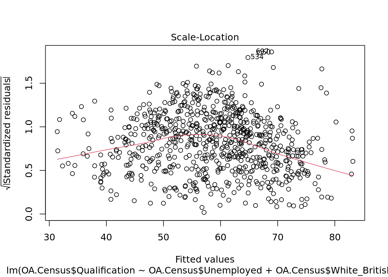
We can also produce a map showing the values of the residuals for each output area in Camden. This might indicate where some parts of the Borough fit the model well and where other parts are not well represented by it.
resids<-residuals(model)

map.resids<-OA.Census

map.resids<- cbind(OA.Census, resids)

# maps the residuals using the quickmap function from tmap
qtm(map.resids, fill = "resids")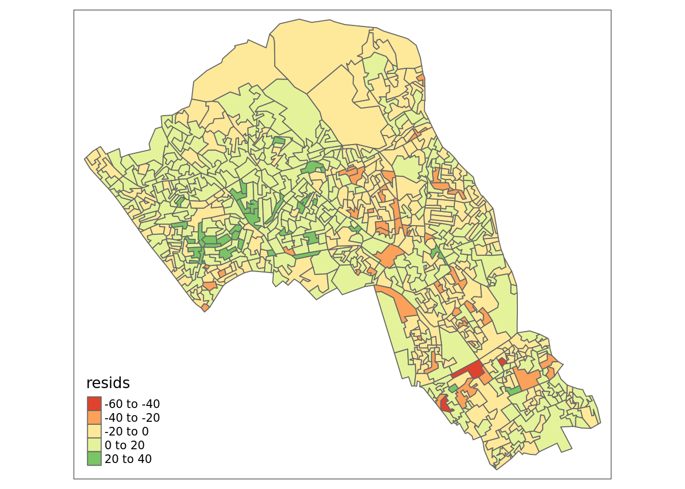
If you notice there is a geographic pattern to the residuals, it is therefore possible that an unobserved variable may also be influencing our dependent variable in the model (% with a qualification) and that some or all of the variables have specific spatial configurations. This is where GWR can help.
Geographically Weighted Regression (GWR)
Some useful extra information can be found here (although a number of links in the further reading no longer work…). The Encyclopedia of Human Geography describes GWR as follows (full entry here):
Geographically weighted regression (GWR) is a local form of spatial analysis introduced into the geographical literature drawing from statistical approaches for curve-fitting and smoothing applications. The method works based on the simple yet powerful idea of estimating local models using subsets of observations centered on a focal point.
Prior to running the model we need to calculate a kernel bandwidth. This will determine now the GWR subsets the data when it tests multiple models across space. Here we specify that we would like to use an adaptive kernel.
library("spgwr")

# The OA.Census object needs to be reformatted to a different type of spatial object in R to work with the spgwr package.

OA.Census.SP<- as(OA.Census, "Spatial")

#calculate kernel bandwidth
GWRbandwidth <- gwr.sel(OA.Census.SP$Qualification ~ OA.Census.SP$Unemployed+OA.Census.SP$White_British, data=OA.Census.SP,adapt=T)

Next we can run the model and view the results.
# run the gwr model
gwr.model = gwr(OA.Census.SP$Qualification ~ OA.Census.SP$Unemployed+OA.Census.SP$White_British, data = OA.Census.SP, adapt=GWRbandwidth, hatmatrix=TRUE, se.fit=TRUE)

#print the results of the model
gwr.model
Upon first glance, much of the outputs are identical to the outputs of the linear model. However we can explore various outputs of this model across each polygon.
We create a results output from the model which contains a number of attributes which correspond which each unique output area from our OA.Census file. In the example below we have printed the names of each of the new variables.
They include a local R2 value, the predicted values (for % qualifications) and local coefficients for each variable. We will then bind the outputs to our OA.Census polygon so we can map them.
results <-as.data.frame(gwr.model$SDF)

names(results)
## [1] "sum.w" "X.Intercept."
## [3] "OA.Census.SP.Unemployed" "OA.Census.SP.White_British"
## [5] "X.Intercept._se" "OA.Census.SP.Unemployed_se"
## [7] "OA.Census.SP.White_British_se" "gwr.e"
## [9] "pred" "pred.se"
## [11] "localR2" "X.Intercept._se_EDF"
## [13] "OA.Census.SP.Unemployed_se_EDF" "OA.Census.SP.White_British_se_EDF"
## [15] "pred.se.1"# Note that this is switching back from the SP to the SF spatial formats.
gwr.map<- OA.Census
gwr.map <- cbind(OA.Census, as.matrix(results))The variable names followed by the name of our original dataframe (i.e. OA.Census.Unemployed) are the coefficients of the model.
qtm(gwr.map, fill = "localR2")
Using gridExtra
We will now consider some of the other outputs. We will create four maps in one image to show the original distributions of our unemployed and White British variables, and their coefficients in the GWR model.
To facet four maps in tmap we can use functions from the grid and gridExtra packages which allow us to split the output window into segments. We will divide the output into four and print a map in each window.
Firstly, we will create four map objects using tmap. Instead of printing them directly as we have done usually, we all assign each map an object ID so it call be called later.
# create tmap objects
map1 <- tm_shape(gwr.map) + tm_fill("White_British", n = 5, style = "quantile")  + tm_layout(frame = FALSE, legend.text.size = 0.5, legend.title.size = 0.6)
map2 <- tm_shape(gwr.map) + tm_fill("OA.Census.SP.White_British", n = 5, style = "quantile", title = "WB Coefficient") + tm_layout(frame = FALSE, legend.text.size = 0.5, legend.title.size = 0.6)
map3 <- tm_shape(gwr.map) + tm_fill("Unemployed", n = 5, style = "quantile") + tm_layout(frame = FALSE, legend.text.size = 0.5, legend.title.size = 0.6)
map4 <- tm_shape(gwr.map) + tm_fill("OA.Census.SP.Unemployed", n = 5, style = "quantile", title = "Ue Coefficient") + tm_layout(frame = FALSE, legend.text.size = 0.5, legend.title.size = 0.6)
With the four maps ready to be printed, we will now create a grid to print them into. From now on every time we wish to recreate the maps we will need to run the grid.newpage() function to clear the existing grid window.
library(grid)
library(gridExtra)
# creates a clear grid
grid.newpage()
# assigns the cell size of the grid, in this case 2 by 2
pushViewport(viewport(layout=grid.layout(2,2)))

# prints a map object into a defined cell
print(map1, vp=viewport(layout.pos.col = 1, layout.pos.row =1))
print(map2, vp=viewport(layout.pos.col = 2, layout.pos.row =1))
print(map3, vp=viewport(layout.pos.col = 1, layout.pos.row =2))
print(map4, vp=viewport(layout.pos.col = 2, layout.pos.row =2))
Multicollinearity
Because GWR builds a local regression equation for each feature in the dataset if there is a clear clustering of explanatory variables – that is they behave in a similar way across space – then you risk local multicollinearity in the analysis. In case you’ve forgotten multicolinearity occurs when two explanatory variables are linearly related and so including them both reduces the explanatory power of each when specifying the model. It can result in inflated variances of regression coefficients, and insignificant statistical test values. We can check for this by examining the correlations between the coefficients produced by the GWR by using the cor() function. Note that the results columns we need are 3,4,6,7, if you have more variables this number will change. Look at the head of the results object to determine what’s needed.
round(cor(results[,c(3,4,6,7)], use ="complete.obs"),2)## OA.Census.SP.Unemployed
## OA.Census.SP.Unemployed 1.00
## OA.Census.SP.White_British 0.03
## OA.Census.SP.Unemployed_se 0.13
## OA.Census.SP.White_British_se 0.23
## OA.Census.SP.White_British
## OA.Census.SP.Unemployed 0.03
## OA.Census.SP.White_British 1.00
## OA.Census.SP.Unemployed_se -0.02
## OA.Census.SP.White_British_se 0.05
## OA.Census.SP.Unemployed_se
## OA.Census.SP.Unemployed 0.13
## OA.Census.SP.White_British -0.02
## OA.Census.SP.Unemployed_se 1.00
## OA.Census.SP.White_British_se 0.60
## OA.Census.SP.White_British_se
## OA.Census.SP.Unemployed 0.23
## OA.Census.SP.White_British 0.05
## OA.Census.SP.Unemployed_se 0.60
## OA.Census.SP.White_British_se 1.00You can also check these as plots.
pairs(results[,c(3,4,6,7)], pch=".")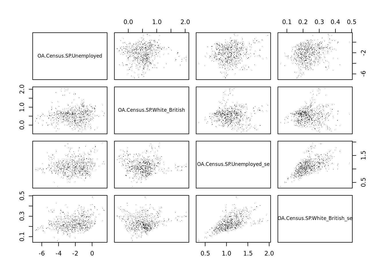
Looking at the above the Unemployed and White British variables don’t appear to be strongly correlated with one another overall and we do not need to worry about the standard errors of each being correlated to the original values. It does appear, however, that the standard errors are correlated with one another and therefore worthy of further investigation – it suggests that there is a trend in where the model is doing well vs where it is not as strong. They might be replaced with an additional variable to see if this remains the case. For more on this see here.
Additional Task
Write a 350 word summary of the analysis you have conducted. Comment on the value of GWR in this context and suggest additional methods that may also be appropriate. Be ready to share this at next week’s seminar.
Reading
This article from the GIS Body of Knowledge gives a very nice overview of GWR, so it is well worth a read.
Geographically Weighted Regression: A Method for Exploring Spatial Nonstationarity: One of the original papers written on the subject.
Geographically Weighted Generalised Linear Modelling: Another clear walk through of GWR – uses a different software package as worked example but as with the above the concepts are well explained.