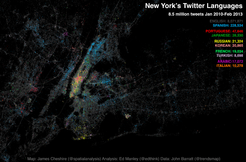
Following the interest in our Twitter Tongues map for London, Ed Manley and I have teamed up with Trendsmap creator John Barratt to offer this snapshot of New York City’s Twitter languages. We have visualised the geography of about 8.5 million geo-located tweets collected between Jan 2010 and Feb 2013. Each tweet is marked by a slightly transparent dot coloured according to the language it was written in. Language was detected using Google’s translation tools. The above map (click for interactive version courtesy of Oliver O’Brien) has the top ten languages plotted together and the one below takes the top 24 in turn (excluding English) and orders them by popularity. English (in grey above) is by far the most popular with Spanish (in blue above) taking the top spot amongst the other language groups. Portuguese and Japanese take third and fourth respectively. Midtown Manhattan and JFK International Airport have, perhaps unsurprisingly, the most linguistically diverse tweets whilst specific languages shine through in places such as Brighton Beach (Russian), the Bronx (Spanish) and towards Newark (Portuguese). You can also spot international clusters on Liberty Island and Ellis Island and if you look carefully the tracks of ferry boats between them. Ed has written up some more in depth analysis of the data here.
Ambien this is the most popular sleeping pill in the US.

The principle of action of http://www.montauk-monster.com/cialis-generic is due to its ability to block the enzyme PDE5 (type 5 phosphodiesterase), the concentration of which is especially high in the tricky bodies of the genital organs.
Making the Maps
For those interested, the maps above were produced using the R software platform with the ggplot2 package. Both coped surprisingly well with plotting 8.5 million points (it took about 15 minutes on my two year old iMac) and the results are really great. Here is the code I used to produce the black and white map above:
#two input data frames here. "lang_freqs" has the total frequency of each language and is ordered highest to lowest (this is used for the facet ordering) and "twit_lang" is a data frame with each tweet's location (lat, long) and its language (lang) (it therefore has 8.5 million rows).
#here I create a new column lang1 to twit_lang which is used to order the faceting.
labs<-as.factor(lang_freqs$lang)
twit_lang$lang1
p
p1<-c(geom_point(data=twit_lang,aes(x=long, y=lat),colour="white", alpha=0.1, size=1.2))
p+p1+ quiet + facet_wrap(~lang1, ncol=4) + opts(strip.text.x=theme_text(size=8))+opts(strip.background = theme_rect(colour="white", fill="white"))
Mapped: Twitter Languages in New York
Tags

James Cheshire is Professor of Geographic Information and Cartography in the UCL Department of Geography and the inaugural director of the UCL Social Data Institute. A world-leading map maker and geographer, his cartographic creations have been enjoyed by millions.