
An Introduction to R
R is a free software environment for statistical computing and graphics. It is extremely powerful and as such is now widely used for academic research as well as in the commercial sector. Unlike software such as Excel or SPSS, the user has to type commands to get it to execute tasks such as loading in a dataset or performing a calculation. The biggest advantage of this approach is that you can build up a document, or script, that provides a record of what you have done, which in turn enables the straightforward repetition of tasks. Graphics can be easily modified and tweaked by making slight changes to the script or by scrolling through past commands and making quick edits. Unfortunately command-line computing can also be off-putting at first. It is easy to make mistakes that aren’t always obvious to detect. Nevertheless, there are good reasons to stick with R. These include:
- It’s broadly intuitive with a strong focus on publishable-quality graphics. It’s ‘intelligent’ and offers in-built good practice – it tends to stick to statistical conventions and present data in sensible ways.
- It’s free, cross-platform, customisable and extendable with a whole swathe of libraries (‘add ons’) including those for discrete choice, multilevel and longitudinal regression, and mapping, spatial statistics, spatial regression and geostatistics.
- It is well respected and used at the world’s largest technology companies (including Google, Microsoft and Facebook), the largest pharmaceutical companies (including Johnson & Johnson, Merck, and Pfizer), and at hundreds of other companies.
- It offers a transferable skill that shows to potential employers experience both of statistics and of computing.
The intention here is to provide an introduction to R. After completing this section you should: 1. Be familiar with the basic programming principles behind R. 2. Be able to load in data from CSV files and subsetting it into smaller chunks. 3. Be able to calculate a number of descriptive statistics for data exploration and checking. 4. Be able to create basic and more complex plots in order to visualise the distributions values within a dataset.
R has a steep learning curve, but the benefits of using it are well worth the effort. Take your time and think through every piece of code you type in. The best way to learn R is to take the basic code provided in tutorials and experiment with changing parameters – such as the colour of points in a graph – to really get “under the hood” of the software. Take lots of notes as you go along and if you are getting really frustrated take a break!
R can be downloaded from https://www.r-project.org/ if it is not on your computer already. Although it is possible to conduct analysis on R directly, you may find it easier to run it via Rstudio which provides a user-friendly graphical user interface. After downloading R, Rstudio can be obtained for free from https://www.rstudio.com/
To open R click on the start menu and open RStudio. You should see a screen resembling the image below (if it prompts you to update just ignore it for now).
ADD IMAGE
It is recommended that you enter your commands into the scripting window of RStudio and use this area as your work space. When you wish to run your commands either hold control Ctrl and enter on your key board for each line or select the line you wish to run and click Run at the top of the scripting window.
The Basics
The example code we use here will be in in boxes like the one below that appear similar to how you should enter them in your rstudio.
At its absolute simplest R is a calculator. If you type the addition below in the command line window, it will give you an answer (after every line you need to hit enter to execute the code).
5+10## [1] 15However, it is often easier to assign numbers (or groups of them) a memorable name. These become objects in R and they are a really important concept. For example:
a<-5
b<-10
The <- symbol is used to assign the value to the name, in the above we assigned the integer 5 to the object a. To see what each object contains you can just type print(name of your object).
print(a)## [1] 5Where the bit in the brackets is the object name. Objects can then be treated in the same way as the numbers they contain. For example:
a*b## [1] 50Or even used to create new objects:
ab<- a*b
print(ab)
## [1] 50You can generate a list of objects that are currently active using the ls() command. R stores objects in your computer’s RAM so they can be processed quickly. Without saving (we will come onto this below) these objects will be lost if you close R (or it crashes).
To show the active R objects type:
ls()## [1] "a" "ab" "b"You may wish to delete an object. This can be done using rm() with the name of the object in the brackets. For example:
rm(ab)Use the ls() command again to see if ab is no longer listed.
ls()## [1] "a" "b"The real power of R comes when we can begin to execute functions on objects. Until now our objects have been extremely simple integers. Now we will build up more complex objects. In the first instance we will use the c() function. “c”” means concatenate and essentially groups things together.
DOB<- c(1993,1993,1994,1991)Type print(DOB) to see the result.
We can now execute some statistical functions on this object
mean(DOB)## [1] 1992.75median(DOB)## [1] 1993range(DOB)## [1] 1991 1994All functions need a series of arguments to be passed to them in order to work. These arguments are typed within the brackets and typically comprise the name of the object (in the examples above its the DOB) that contains the data followed by some parameters. The exact parameters required are listed in the functions help files. To find the help file for the function type() ? followed by the function name, for example: ?mean
All helpfiles will have a “Usage” heading detailing the parameters required. In the case of the mean you can see it simply says mean(x, ...). In function helpfiles x will always refer to the object the function requires and, in the case of the mean, the “…” refers to some optional arguments that we don’t need to worry about.
When you are new to R the help files can seem pretty impenetrable (because they often are!). Up until relatively recently these were all people had to go on, but in recent years R has really taken off and so there are plenty of places to find help and tips. Google is best tool to use. When people are having problems they tend to post examples of their code online and then the R community will correct it. One of the best ways to solve a problem is to paste their correct code into your R command line window and then gradually change it for your data an purposes.
The structure of the DOB object – essentially a group of numbers – is known as a vector object in R. To build more complex objects that, for example, resemble a spreadsheet with multiple columns of data, it is possible to create a class of objects known as a data frame. This is probably the most commonly used class of object in R. We can create one here by combining two vectors.
singers <- c("Zayn", "Liam", "Harry", "Louis")
one_direction <- data.frame(singers, DOB)
If you type print(one_direction) you will see our data frame.
print(one_direction)## singers DOB
## 1 Zayn 1993
## 2 Liam 1993
## 3 Harry 1994
## 4 Louis 1991Tips
- R is case sensitive so you need to make sure that you capitalise everything correctly.
- The spaces between the words don’t matter but the positions of the commas and brackets do. Remember, if you find the prompt, >, is replaced with a + it is because the command is incomplete. If necessary, hit the escape (esc) key and try again.
- It is important to come up with good names for your objects. In the case of the One.Direction object I used a full-stop to separate the words as well as capitilisation. It is good practice to keep the object names as short as posssible so I could have gone for OneDirection or one.dir. You cannot start an object name with a number so 1D won’t work.
- If you press the up arrow in the command line you will be able to edit the previous lines of code you inputted.
Working with data In the previous section, R may have seemed fairly labour-intensive. We had to enter all our data manually and each line of code had to be written into the command line. Fortunately this isn’t routinely the case. In R Studio look to the top left corner and you will see a plus symbol, click on it and select “R Script”. This should give you a blank document that looks a bit like the command line. The difference is that anything you type here can be saved as a script and re-run at a later date. When writing a script it is important to keep notes about what each step is doing. To do this the hash # symbol is put before any code. This comments out that particular line so that R ignores it when the script is run. Type the following into the script:
#This is my first R script
My.Data<- data.frame(0:10, 20:30)
print(My.Data)
## X0.10 X20.30
## 1 0 20
## 2 1 21
## 3 2 22
## 4 3 23
## 5 4 24
## 6 5 25
## 7 6 26
## 8 7 27
## 9 8 28
## 10 9 29
## 11 10 30In the scripting window if you highlight all the code you have written and press the “Run” button on the top on the scripting window you will see that the code is sent to the command line and the text on the line after the # is ignored. From now on you should type your code in the scripting window and then use the Run button to execute it. If you have an error then edit the line in the script and hit run again. The My.Data object is a data frame in need of some sensible column headings. You can add these by typing:
#Add column names
names(My.Data)<- c("X", "Y")

#print My.Data object to check names were added successfully.
print(My.Data)
## X Y
## 1 0 20
## 2 1 21
## 3 2 22
## 4 3 23
## 5 4 24
## 6 5 25
## 7 6 26
## 8 7 27
## 9 8 28
## 10 9 29
## 11 10 30Until now we have generated the data used in the examples above. One of R’s great strengths is its ability to load in data from almost any file format. Comma Separated Value (CSV) files are our preferred choice. These can be thought of as stripped down Excel spreadsheets. They are an extremely simple format so they are easily machine readable and can therefore be easily read in and written out of R. Since we are now reading and writing files it is good practice to tell R what your working directory is.
This is the folder on the computer where you wish to store the data files you are working with. You can create a folder called “POLS0008” for example. If you are using RStudio, on the lower right of the screen is a window with a “Files” tab. If you click on this tab you can then navigate to the folder you wish to use. You can then click on the “More” button and then “Set as Working Directory”. You should then see some code similar to the below appear in the command line. It is also possible to type the code in manually.
#Set the working directory. The bit between the "" needs to specify the path to the folder you wish to use (you will see my file path below).  You may need to create the folder first.

setwd("~/POLS0008") # Note the single / (\\ will also work).
Once the working directory is setup it is then possible to load in a csv file. We are going to load a dataset that has been saved in the working directory we just set that shows London’s historic population for each of its Boroughs. You need to download this dataset from Moodle. Link here or go to Week 1 and download the files from there: https://moodle-1819.ucl.ac.uk/mod/resource/view.php?id=488388.
This file will then need to be uploaded into RStudio. To do this click on the “Upload” button in the files area of the screen. Select the zipfile and press OK. The folder “pracs1-3” should appear and if you click on it you can see there are two files. Press the green up arrow (or the small dots next to it) to return to your working directory. We can then type the following to locate and load in the file we need.
#load in csv file
pop<- read.csv("worksheet_data/Intro/census-historic-population-borough.csv")
To view the object type:
print(pop)Or if you only want to see the top 10 or bottom 10 rows you can use the head() and tail() commands. These are particularly useful if you have large datasets.
head(pop)tail(pop)To get to know a bit more about the file you have loaded R has a number of useful functions. We can use these to find out how many columns (variables) and rows (cases) the data frame (dataset) contains.
#Get the number of columns

ncol(pop)
## [1] 25## [1] 25
#Get the number of rows
nrow(pop)## [1] 33## [1] 33
#List the column headings
names(pop)Given the number of columns in the pop data frame, subsetting by selecting on the columns of interest would make it easier to handle. In R there are two was of doing this. The first uses the $ symbol to select columns by name and then create a new data frame object.
#Select the columns containing the Borough names and the 2011 population.

pop.2011<- data.frame(pop$Area.Name, pop$Persons.2011)

head(pop.2011)
## pop.Area.Name pop.Persons.2011
## 1 City of London 7375
## 2 Barking and Dagenham 185911
## 3 Barnet 356386
## 4 Bexley 231997
## 5 Brent 311215
## 6 Bromley 309392A second approach to selecting particular data is to use [Row, Column].
pop[1,2]## [1] "City of London"pop[1:5,1]## [1] "00AA" "00AB" "00AC" "00AD" "00AE"pop[1:5, 8:11]## Persons.1851 Persons.1861 Persons.1871 Persons.1881
## 1 128000 112000 75000 51000
## 2 8000 8000 10000 13000
## 3 15000 20000 29000 41000
## 4 12000 15000 22000 29000
## 5 5000 6000 19000 31000#Assign the previous selection to a new object
pop.subset<- pop[1:5, 8:11]In the code snippet, note how the colon : is used to specify a range of values. We used the same technique to create the My.Data object above. The abilty to select particular columns means we can see how the population of London’s Boroughs have changed over the past century.
#Within the brackets you can add additional columns to the data frame so long as their separated by commas
PopChange<- data.frame(pop$Area.Name, pop$Persons.2011 - pop$Persons.1911)
If you type head(PopChange) you will see that the population change column (created to the right of the comma above) has a very long name. This can be changed using the names() command.
names(PopChange)<- c("Borough", "Change_1911_2011")Since we have done some new analysis and created additional information it would be good to save the PopChange object to our working directory. This is done using the code below. Within the brackets we put the name of the R object we wish to save on the left of the comma and the file name on the right of the comma (this needs to be in inverted commas). Remember to put “.csv” after since this is the file format we are saving in.
write.csv(PopChange, "worksheet_data/Population_Change_1911_2011.csv")Task
Create a CSV file that contains the following columns: 1. The names of the London Boroughs 2. Population change between 1811 and 1911 3. Population change between 1911 and 1961 4. Population change 1961 and 2011
Which Boroughs had the fastest growth during the 19th Century, and which had the slowest?
You may have noticed that there is an additional column in the pop data frame called Borough-Type. This indicates if a Borough is in inner (1) or outer (2) London. Is this variable ordinal or nominal? Save your R script by pressing the Save button in the script window.
Getting to Know Your Data: Descriptive Statistics and Plots
For this tutorial we will continue to use the pop object created in the previous section. You may still have it loaded into your R workspace. To check if you do you can use the ls() command. Type this into the command line and see if pop is printed. If not you can simply reload it:
#first set your working directory as before, remember your file path may be different to mine.

#setwd("~/Intro_R")

#load in csv file
pop<- read.csv("worksheet_data/Intro/census-historic-population-borough.csv")
Use the head() command to remind yourself of the structure of the pop data frame. You should see 25 columns of data.
Plotting Data with R
Tools to create high quality plots have become one of R’s greatest assets. This is a relatively recent development, since the software has traditionally been focused on the statistics rather than visualisation. The standard installation of R has base graphic functionality built in to produce very simple plots. For example we can plot the relationship between the London population in 1811 and 1911.
#left of the comma is the x-axis, right is the y-axis. Also note how we are using the $ command to select the columns of the data frame we want.

plot(pop$Persons.1811,pop$Persons.1911)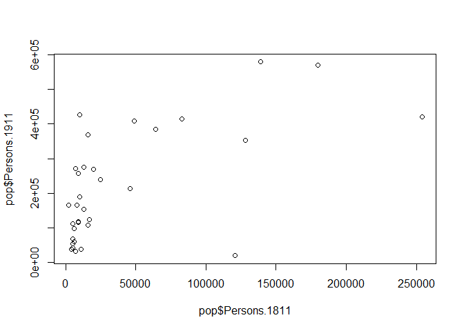
You should see a very simple scatter graph. The plot command offers a huge number of options for customisation. You can see them using the ?plot help pages and also the ?par help pages (par in this case is short for parameters). There are some examples below (note how the parameters come after the x and y columns).
#Add a title, change point colour, change point size

plot(pop$Persons.1811,pop$Persons.1911, main="My first R plot", col="blue", cex=2)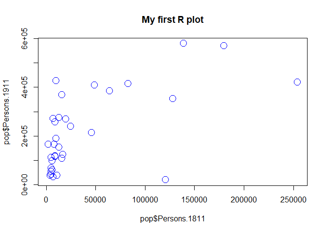
#Add a title, change point colour, change point symbol

plot(pop$Persons.1811,pop$Persons.1911, main="My first R plot", col="magenta", pch=22)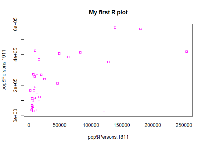
For more information on the plot parameters (some have obscure names) see here: http://www.statmethods.net/advgraphs/parameters.html
ggplot2
A slightly different method of creating plots in R requires the ggplot2 package. There are many hundreds of packages in R each designed for a specific purpose. These are not installed automatically, so each one has to be downloaded and then we need to tell R to use it. To download and install the ggplot2 package type the following:
#When you hit enter R will ask you to select a mirror to download the package contents from. It doesn't really matter which one you choose, I tend to pick the UK based ones.

install.packages("ggplot2")
The install.packages step only needs to be performed once. You don’t need to install a the package every time you want to use it. However, each time you open R and wish to use a package you need to use the library() command to tell R that it will be required.
library("ggplot2")The package is an implementation of the Grammar of Graphics (Wilkinson 2005) – a general scheme for data visualisation that breaks up graphs into semantic components such as scales and layers. ggplot2 can serve as a replacement for the base graphics in R and contains a number of default options that match good visualisation practice.
Whilst the instructions are step by step you are encouraged to deviate from them (trying different colours for example) to get a better understanding of what we are doing. For further help, ggplot2 is one of the best documented packages in R and has an extensive website: http://docs.ggplot2.org/current/. Good examples of graphs can also be found on the website cookbook-r.com.
p <- ggplot(pop, aes(Persons.1811, Persons.1911))What you have just done is set up a ggplot object where you say where you want the input data to come from – in this case it is the pop object. The column headings within the aes() brackets refer to the parts of that data frame you wish to use (the variables Persons.1811 and Persons.1911). aes is short for ‘aesthetics that vary’ – this is a complicated way of saying the data variables used in the plot. If you just type p and hit enter you get the error No layers in plot. This is because you have not told ggplot what you want to do with the data. We do this by adding so-called geoms, in this case geom_point(), to create a scatter plot.
p + geom_point()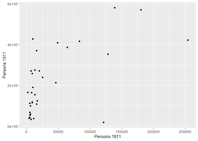
You can already see that this plot is looking a bit nicer than the one we created with the base plot() function used above. Within the geom_point() brackets you can alter the appearance of the points in the plot. Try something like p + geom_point(colour = "red", size=2) and also experiment with your own colours/ sizes. If you want to colour the points according to another variable it is possible to do this by adding the desired variable into the aes() section after geom_point(). Here will indicate the size of the population in 2011 as well as the relationship between in the size of the population in 19811 and 1911.
p + geom_point(aes(colour = Persons.2011, size = 2))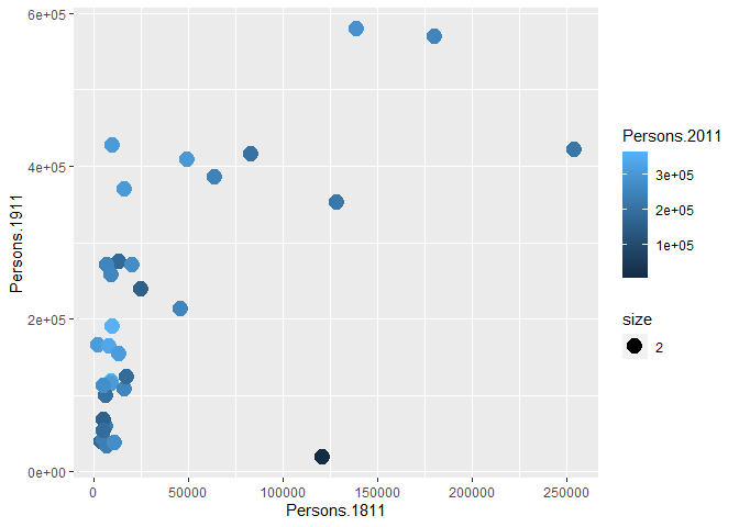
You will notice that ggplot has also created a key that shows the values associated with each colour. In this slightly contrived example it is also possible to resize each of the points according to the Persons.2011 variable.
p + geom_point(aes(size = Persons.2011))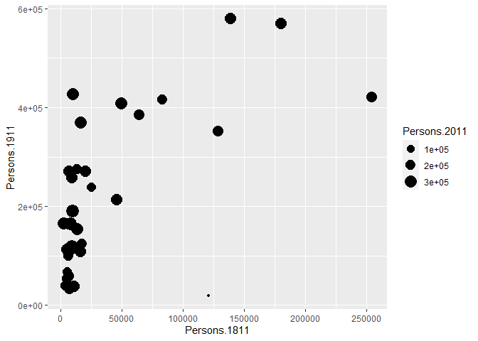
The real power of ggplot2 lies in its ability build a plot up as a series of layers. This is done by stringing plot functions (geoms) together with the + sign. In this case we can add a text layer to the plot using geom_text().
p + geom_point(aes(size = Persons.2011)) + geom_text(size = 2,colour="red",
    aes(label = Area.Name))
This idea of layers (or geoms) is quite different from the standard plot functions in R, but you will find that each of the functions does a lot of clever stuff to make plotting much easier (see the ggplot2 documentation for a full list). The above code adds London Borough labels to the plot over the points they correspond to. This isn’t perfect since many of the labels overlap but they serve as a useful illustration of the layers. To make things a little easier the plot can be saved as a PDF using the ggsave command. When saving the plot can be enlarged to help make the labels more legible.
ggsave(filename = "first_ggplot.pdf", plot = p, scale=2)ggsave only works with plots that were created with ggplot. Within the brackets you should create a file name for the plot – this needs to include the file format (in this case .pdf you could also save the plot as a .jpg file). The file will be saved to your working directory. The scale controls how many times bigger you want the exported plot to be than it currently is in the plot window. Once executed you should be able to see a PDF file in your working directory.
Quick Recap
The previous section covered: 1. The creation of scatter plots using the base plot functionality in R. 2. Installing and loading additional packages in R. 3. The basics of the ggplot2 package for creating plots including: 1. Plot layers (geoms) 2. Where to specific the data variables (within the aes() brackets) 3. Saving your plot.
Describing Data – Statistics
In addition to plotting, descriptive statistics offer a further tool for getting to know your data. They provide useful summaries of a dataset and along with intelligent plotting can also provide a good “sanity check” to ensure the data conform to expectations. For the rest of this tutorial we will change our dataset to one containing the number of assault incidents that ambulances have been called to in London between 2009 and 2011. You will need to download a revised version of this file from Moodle: ambulance_assault.csv and upload it to your working directory (replace your existing file). It is in the same data format (CSV) as our London population file so we use the read.csv() command.
#read in the ambulance_assault datafile

input <- read.csv("worksheet_data/Intro/ambulance_assault.csv")

#Check that the data have been loaded in correctly we can see the top 6 rows with the head() command.

head(input)
## Bor_Code WardName WardCode WardType assault_09_11
## 1 00AA Aldersgate 00AAFA Prospering Metropolitan 10
## 2 00AA Aldgate 00AAFB Prospering Metropolitan 0
## 3 00AA Bassishaw 00AAFC Prospering Metropolitan 0
## 4 00AA Billingsgate 00AAFD Prospering Metropolitan 0
## 5 00AA Bishopsgate 00AAFE Prospering Metropolitan 188
## 6 00AA Bread Street 00AAFF Prospering Metropolitan 0#To get a sense of how large the data frame is, look at how many rows you have
nrow(input)## [1] 649You will notice that the data table has 4 columns and 649 rows. The column headings are abbreviations of the following: You will notice that the data table has 4 columns and 649 rows. The column headings are abbreviations of the following: Bor_Code: Borough Code. London has 32 Boroughs (such as Camden, Islington, Westminster etc) plus the City of London at the centre. These codes are used as a quick way of referring to them from official data sources. WardName: Boroughs can be broken into much smaller areas known as Wards. These are electoral districts and have existed in London for centuries. WardCode: A statistical code for the Wards above. WardType: a classification that groups wards based on similar characteristics. assault_09_11: The number of assault incidents requiring an ambulance between 2009 and 2011 for each Ward. The mean(), median() and range() were some of the first R functions we used at the last week to describe our One.Direction dataset. We will use these to describe our assaults data as well as other descriptive statistics, including standard deviation.
#Calculate the mean of the assaults variable:

mean(input$assault_09_11)
## [1] 173.4669## [1] 173.5
#Calculate the standard deviation of the assaults variable:
sd(input$assault_09_11)## [1] 130.3482## [1] 130.3
#Calculate the range, first starting by calculating the minimum and maximum values:
min(input$assault_09_11)## [1] 0## [1] 0
max(input$assault_09_11)## [1] 1582## [1] 1582
range(input$assault_09_11)## [1] 0 1582## [1] 0 1582These are commonly used descriptive statistics. To make things even easier, R has a summary() function that calculates a number of these routine statistics simultaneously.
summary(input$assault_09_11)## Min. 1st Qu. Median Mean 3rd Qu. Max.
## 0.0 86.0 146.0 173.5 233.0 1582.0You should see you get the minimum (Min.) and maximum (Max.) values of the assault_09_11 column; its first (1st Qu.) and third (3rd Qu.) quartiles that comprise the interquartile range; its the mean and the median. The built-in R summary() function does not calculate the standard deviation. There are functions in other libraries that calculate more detailed descriptive statistics, including describe() in the psych package , which we will use in the later tutorials. We can also use the summary() function to describe a categorical variable and it will list its levels:
summary(input$WardType)## Length Class Mode
## 649 character character#We can create the same output by creating a frequency table using the table() function
freqtable<-table(input$WardType)
freqtable#To find the table of proportion we can use the prop.table() function
prop.table(freqtable)Explain why each of these statistics are useful below and what type of data are required to calculate them: Mean: Median: Mode: Interquartile Range: Range: Standard Deviation:
Describing Data – Plots
Here we pick up where we left off in the previous section. If you have closed R then you will need to reload your data.
#Here we reload the object - note that the file path will be different for your own system so should be adjusted accordingly.

input <- read.csv("worksheet_data/camden/ambulance_assault.csv")
Through plotting we can provide graphical representations of the data to support the statistics above. To simply have the Ward codes on the x-axis and their assault values on the y-axis we need to plot the relevant columns of the input object.
Histograms
The basic plot created in the previous step doesn’t look great and it is hard to interpret the raw assault count values. A frequency distribution plot in the form of a histogram will be better. You will learn more about frequency distributions next week so just for now we will focus on generating the plots. There are many ways to do this in R but we will use the functions contained within the ggplot2 library.
library(ggplot2)

p_ass <- ggplot(input, aes(x=assault_09_11))
The ggplot(input, aes(x=assault_09_11)) section means create a generic plot object (called p.ass) from the input object using the assault_09_11 column as the data for the x axis. Remember the data variables are required as aesthetics parameters so the assault_09_11 appears in the aes() brackets. Histograms provide a nice way of graphically summarising a dataset. To create the histogram you need to add the relevant ggplot2 command (geom).
p_ass +
  geom_histogram()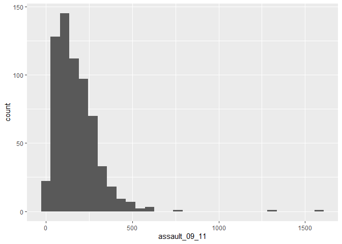
## stat_bin: binwidth defaulted to range/30. Use 'binwidth = x' to adjust this.The height of each bar (the x-axis) shows the count of the datapoints and the width of each bar is the value range of datapoints included. If you want the bars to be thinner (to represent a narrower range of values and capture some more of the variation in the distribution) you can adjust the binwidth. Binwidth controls the size of ‘bins’ that the data are split up into. We will discuss this in more detail later in the course, but put simply, the bigger the bin (larger binwidth) the more data it can hold. Try:
p_ass +
  geom_histogram(binwidth=10) +
geom_density(fill=NA, colour="black") 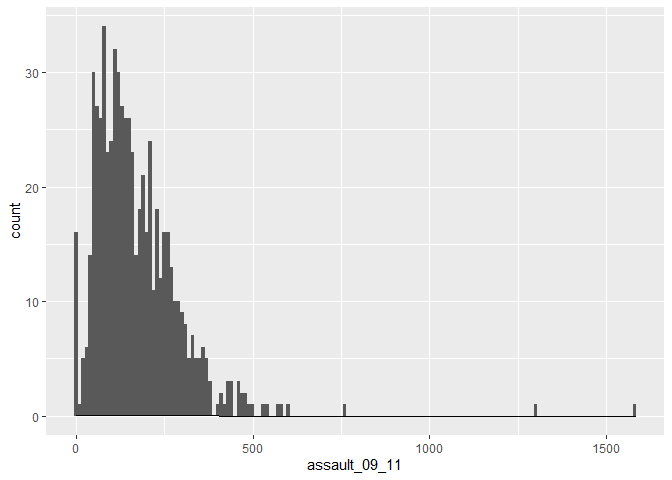
You can also overlay a density distribution over the top of the histogram. Again, this will be discussed in more detail next week, but think of the plotted line as a summary of the underlying histogram. For this we need to produce a second plot object that says we wish to use the density distribution as the y variable.
p2_ass <- ggplot(input, aes(x=assault_09_11, y=..density..))

p2_ass +
  geom_histogram() +
  geom_density(fill=NA, colour="red")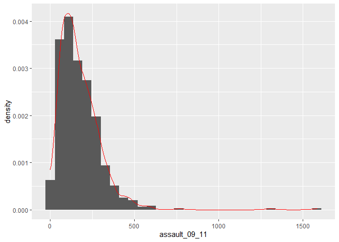
## stat_bin: binwidth defaulted to range/30. Use 'binwidth = x' to adjust this.This plot has provided a good impression of the overall distribution, but it would be interesting to see characteristics of the data within each of the Boroughs. We can do this since each Borough in the input object is made up of multiple wards. To see what I mean, we can select all the wards that fall within the Borough of Camden, which has the code 00AG (if you want to see what each Borough the code corresponds to, and learn a little more about the statistical geography of England and Wales, then see here: http://en.wikipedia.org/wiki/ONS_coding_system).
camden <- input[input$Bor_Code=="00AG",]The crucial part of the code snippet above is what’s included in the square brackets [ ]. We are subsetting the input object, but instead of telling R what column names or numbers we require, we are requesting all rows in the Bor_Code column that contain00AG. 00AG is a text string so it needs to go in speech marks “” and we need to use two equals signs == in R to mean “equals to”. A single equals sign = is another way of assigning objects (it works the same way as <- but is much less widley used for this purpose because it is used when paramaterising functions). So to produce Camden’s frequency distribution the code above needs to be replicated using the camden object in the place of input
p_ass_camden <- ggplot(camden, aes(x=assault_09_11))

p_ass_camden +
geom_histogram() 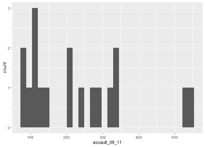
## stat_bin: binwidth defaulted to range/30. Use 'binwidth = x' to adjust this.#We can also add a title using the ggtitle() option
p_ass_camden +
geom_histogram() +
ggtitle("Camden Assault")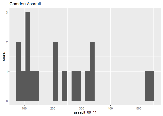
## stat_bin: binwidth defaulted to range/30. Use 'binwidth = x' to adjust this.As you can see this looks a little different from the density of the entire dataset. This is largely becasue we have relatively few rows of data in the camden object (use nrow(camden) to find out just how many). Nevertheless it would be interesting to see the data distributions for each of the London Boroughs. It is a chance to use the facet_wrap() function in R. This brilliant function lets you create a whole load of graphs at once.
#note that we are back to using the p.ass ggplot object since we need all our data for this. This code may generate a large number of warning messages relating to the plot binwidth, don't worry about them.
p_ass +
geom_histogram() +
facet_wrap(~Bor_Code)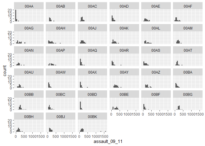 …or you could use
 facet_wrap() to plot according to WardType. What are the key differences in the distributions between the different types?
p_ass +
  geom_histogram() +
  facet_wrap(~WardType)
The facet_wrap() part of the code simply needs the name of the column you would like to use to subset the data into individual plots. Before the column name a tilde ~ is used as shorthand for “by” – so using the function we are asking R to facet the input object into lots of smaller plots based on the Bor_Code column in the first example and WardType in the second. Use the facet_wrap() help file to learn how to create the same plot but with the graphs arranged into 4 columns.
Box and Whisker Plots
In addition to histograms, a type of plot that shows the core characteristics of the distribution of values within a dataset, and includes some of the summary() information we generated earlier, is a box and whisker plot (boxplot for short). These too can be easily produced in R. The diagram below illustrates the components of a box and whisker plot. How these relate to the frequency distribution plots we created above will be explored next week.
INSERT IMAGE
We can create a third plot object for this from the input object:
#note that the `assault_09_11` column is now y and not x and that we have specified x=1. This aligns the plot to the x-axis (any single number would work)

p3_ass <- ggplot(input, aes(x=1, y=assault_09_11))
And then convert it to a boxplot using the geom_boxplot() command.
p3_ass +
  geom_boxplot()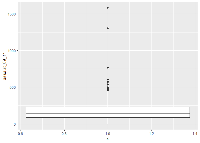
If we are just interested in Camden then we can use the camden object created above in the code.
p3_ass_camden <- ggplot(camden, aes(x=1, y=assault_09_11))

p3_ass_camden +
  geom_boxplot()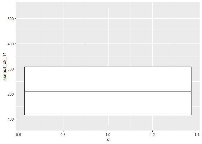
#If you prefer you can flip the plot 90 degrees so that it reads from left to right.

p3_ass_camden +
  geom_boxplot()+
  coord_flip()
You can see that Camden looks a little different to the boxplot of the entire dataset. It would therefore be useful to compare the distributions of data within each of the Boroughs in a single plot as we did with the frequency distributions above. ggplot makes this very easy, we just need to change the x= parameter to the Borough code column (Bor_Code).
p4_ass <- ggplot(input, aes(x=Bor_Code, y=assault_09_11))

p4_ass +
  geom_boxplot()+
  coord_flip()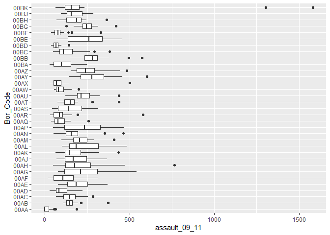
Task
Take census-historic-population-borough.csv file we used to produce the scatter plots of London’s population and create 3 different types of plot from one or more of the variables.
Data Preparation
We are going to open three different datasets from the 2011 Census for the remainder of the sessions. Each file contains data collected from the Census and reported at the ‘Output Area’ level. You will see what Output Areas are later in the course when you come to map the data but essentially they are small areas that very approximately contain 250 people. So each row in our table contains data on how many people have the attribute we are interested in, or what percentage of the population of that area share that attribute.
We can read CSVs into R using the read.csv() function. This requires us to identify the file location within our workspace, and also assign an object name for our data in R.
In the ‘datasets_description.csv’ file you can see the full list of the table names and what they contain. All the census data for Camden have been included in this folder should you wish to explore the data in more detail after you have completed the worksheet steps.
# read.csv() loads a csv, remember to correctly input the file location within your working directory
ethnicity <- read.csv("worksheet_data/camden/KS201EW_oa11.csv")
rooms <- read.csv("worksheet_data/camden/KS403EW_oa11.csv")
qualifications <-read.csv("worksheet_data/camden/KS501EW_oa11.csv")
employment <-read.csv("worksheet_data/camden/KS601EW_oa11.csv")
Viewing data
With the data now loaded into RStudio, they can be observed in the objects window. Alternatively, you can open them with the View function as demonstrated below.
# to view the top 1000 cases of a data frame
View(employment)
All functions need a series of arguments to be passed to them in order to work. These arguments are typed within the brackets and typically comprise the name of the object (in the examples above its the DOB) that contains the data followed by some parameters. The exact parameters required are listed in the functions’ help files. To find the help file for the function type ? followed by the function name, for example – ?View
There are two problems with the data. Firstly, the column headers are still codes and are therefore uninformative. Secondly, the data is split between three different data objects.
First let’s reduce the data. The tables contain both raw population counts and also percentages. We will be working with the percentages as the populations of Output Areas are not identical across our sample.
Observing column names
To observe the column names for each dataset we can use a simple names() function. It is also possible to work out their order in the columns from observing the results of this function.
# view column names of a dataframe
names(employment)
## [1] "GeographyCode" "KS601EW0001" "KS601EW0002" "KS601EW0003"
## [5] "KS601EW0004" "KS601EW0005" "KS601EW0006" "KS601EW0007"
## [9] "KS601EW0008" "KS601EW0009" "KS601EW0010" "KS601EW0011"
## [13] "KS601EW0012" "KS601EW0013" "KS601EW0014" "KS601EW0015"
## [17] "KS601EW0016" "KS601EW0017" "KS601EW0018" "KS601EW0019"
## [21] "KS601EW0020" "KS601EW0021" "KS601EW0022" "KS601EW0023"
## [25] "KS601EW0024" "KS601EW0025" "KS601EW0026" "KS601EW0027"
## [29] "KS601EW0028" "KS601EW0029"From using the variables_description csv in the data folder, we know the Economically active: Unemployed percentage variable is recorded as KS601EW0017. This is the 19th column in the employment dataset.
Selecting columns
Next we will create new data objects which only include the columns we require. The new data objects will be given the same object name as the original one we created when we loaded in the data. Doing so will overwrite the bigger table object in the R session. Using the variable_description csv to lookup the codes, we have isolated only the columns we are interested in. Remember we are working with percentages, not raw counts.
# selecting specific columns only
# note this action overwrites the labels you made for the original data,
# so if you make a mistake you will need to reload the data into R
ethnicity <- ethnicity[, c(1, 21)]
rooms <- rooms[, c(1, 13)]
employment <- employment[, c(1, 20)]
qualifications <- qualifications[, c(1, 20)]
Renaming column headers
Next we want to change the names of the codes to ease our interpretation. We can do this using names().
If we wanted to change an individual column name we could follow the approach detailed below. In this example, we tell R that we are interested in setting the name Unemployed to the 2nd column header in the data.
# to change an individual column name
names(employment)[2] <- "Unemployed"
However, we want to name both column headers in all of our data. To do this we can enter the following code. Remember from our example above, the c() function allows us to concatenate multiple values within one command.
# to change both column names

names(ethnicity)<- c("OA", "White_British")
names(rooms)<- c("OA", "Low_Occupancy")
names(employment)<- c("OA", "Unemployed")
names(qualifications)<- c("OA", "Qualification")
Joining data in R
We next want to combine the data into a single dataset. Joining two data frames together requires a common field, or column, between them. In this case it is the OA field (OA is short for Output Area). In this field each OA has a unique ID (or OA name), these IDs can be used to identify each OA between each of the datasets.
In R the merge() function joins two datasets together and creates a new object. As we are seeking to join four datasets we need to undertake multiple steps as follows.
#1 Merge Ethnicity and Rooms to create a new object called "merged_data_1"
merged_data_1 <- merge(ethnicity, rooms, by="OA")

#2 Merge the "merged_data_1" object with Employment to create a new merged data object
merged_data_2 <- merge(merged_data_1, employment, by="OA")

#3 Merge the "merged_data_2" object with Qualifications to create a new data object
census_data <- merge(merged_data_2, qualifications, by="OA")

#4 Remove the "merged_data" objects as we won't need them anymore
rm(merged_data_1, merged_data_2)
Our newly formed census_data object contains all four variables.
Exporting Data
You can now save this file to your workspace folder. Remember R is case sensitive so take note of when object names are capitalised.
# Writes the data to a csv named "practical_data" in your file directory
write.csv(census_data, "worksheet_data/camden/practical_data.csv", row.names=F)