Less is More: Data Visualisations for Big Data


 I recently stumbled upon a great dataset. It’s the first to provide comprehensive data for world city sizes as far back as 3700BC. The authors (Meredith Reba, Femke Reitsma & Karen Seto) write:
How were cities distributed globally in the past? How many people lived in these cities? How did cities influence their local and regional environments? In order to understand the current era of urbanization, we must understand long-term historical urbanization trends and patterns. However, to date there is no comprehensive record of spatially explicit, historic, city-level population data at the global scale. Here, we developed the first spatially explicit dataset of urban settlements from 3700 BC to AD 2000, by digitizing, transcribing, and geocoding historical, archaeological, and census-based urban population data previously published in tabular form by Chandler and Modelski.
These kinds of data are crying out to be mapped so that’s what I did…
Read more (and get the R code)
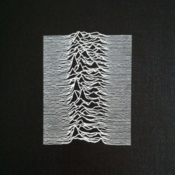
There has been a resurgence of interest in data visualizations inspired by Joy Division’s Unknown Pleasures album cover. These so-called “Joy Plots” are easier to create thanks to the development of the “ggjoy” R package and also some nice code posted using D3. I produced a global population map (details here) using a similar technique in 2013 and since then I’ve been on a quest to find some earlier examples. This is because a number of people have said it reminds them of maps created by Harvard’s digital mapping pioneers in the 1970s and I got the feeling I was coming late to the party…
The pulsar style plots are already well covered by Jen Christiansen who wrote an excellent blog post about the Joy Division album cover, which includes many examples in a range of scientific publications and also features this interview with the designer Peter Saville.
Most interestingly, Jen’s post also includes the glimpse of the kind of map (top left) that I’d heard about but have been unable to get my hands on shown in the book Graphis Diagrams: The Graphic Visualization of Abstract Data.

My luck changed this week thanks to a kind email from John Hessler (Specialist in Mathematical Cartography and GIS at the Library of Congress) alerting me to the huge archive of work they have associated with GIS pioneer Roger Tomlinson (who’s PhD thesis I feature here). I enquired if he knew anything about the population lines maps to which he causally replied “we have hundreds of those” and that he’d already been blogging extensively on the early GIS/ spatial analysis pioneers (I’ve posted links below).
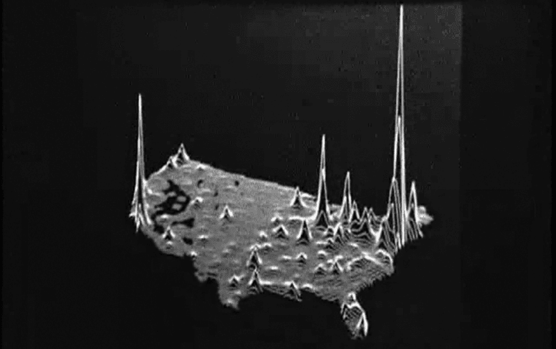
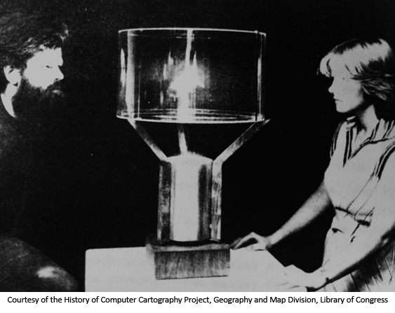
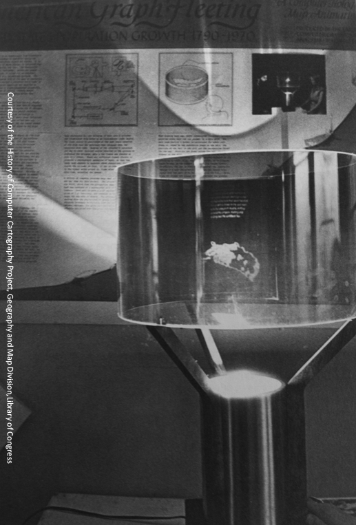
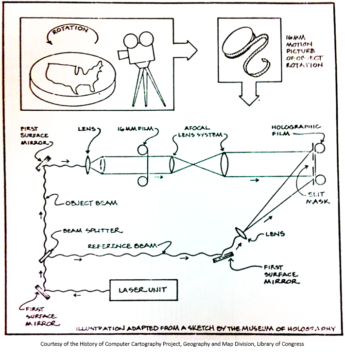
John sent me the below movie entitled “American Graph Fleeting, United States Population Growth 1790-1970” created in 1978. It’s extraordinary, both in how contemporary it looks but also because it was created as a hologram!
The late Roger Tomlinson is considered the “Father of Geographic Information Systems” and he completed his PhD in the UCL Department of Geography in 1974. Tomlinson pioneered digital mapping – every map created using a computer today still uses the principles he laid down in his thesis and its associated work creating the “The Canada Geographic Information System“. I’m pleased to say that after over four decades of sitting on a shelf within the department we now have it fully digitised (and OCRed so it’s searchable) and available to download here.
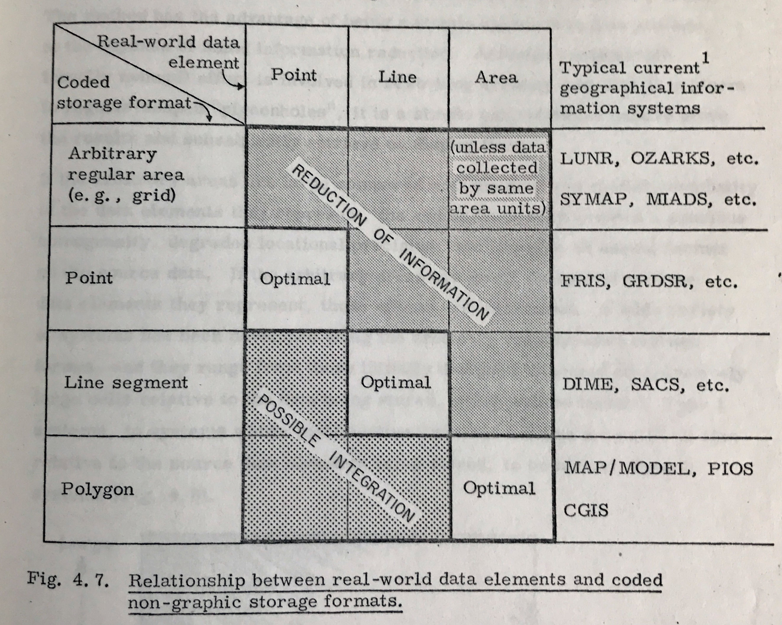
The thesis is entitled “Geographical Information Systems, Spatial Data Analysis and Decision Making in Government” and it’s remarkably timeless in its content. So many of Tomlinson’s principles apply today – not just in his conception of the flow and types of spatial data elements…

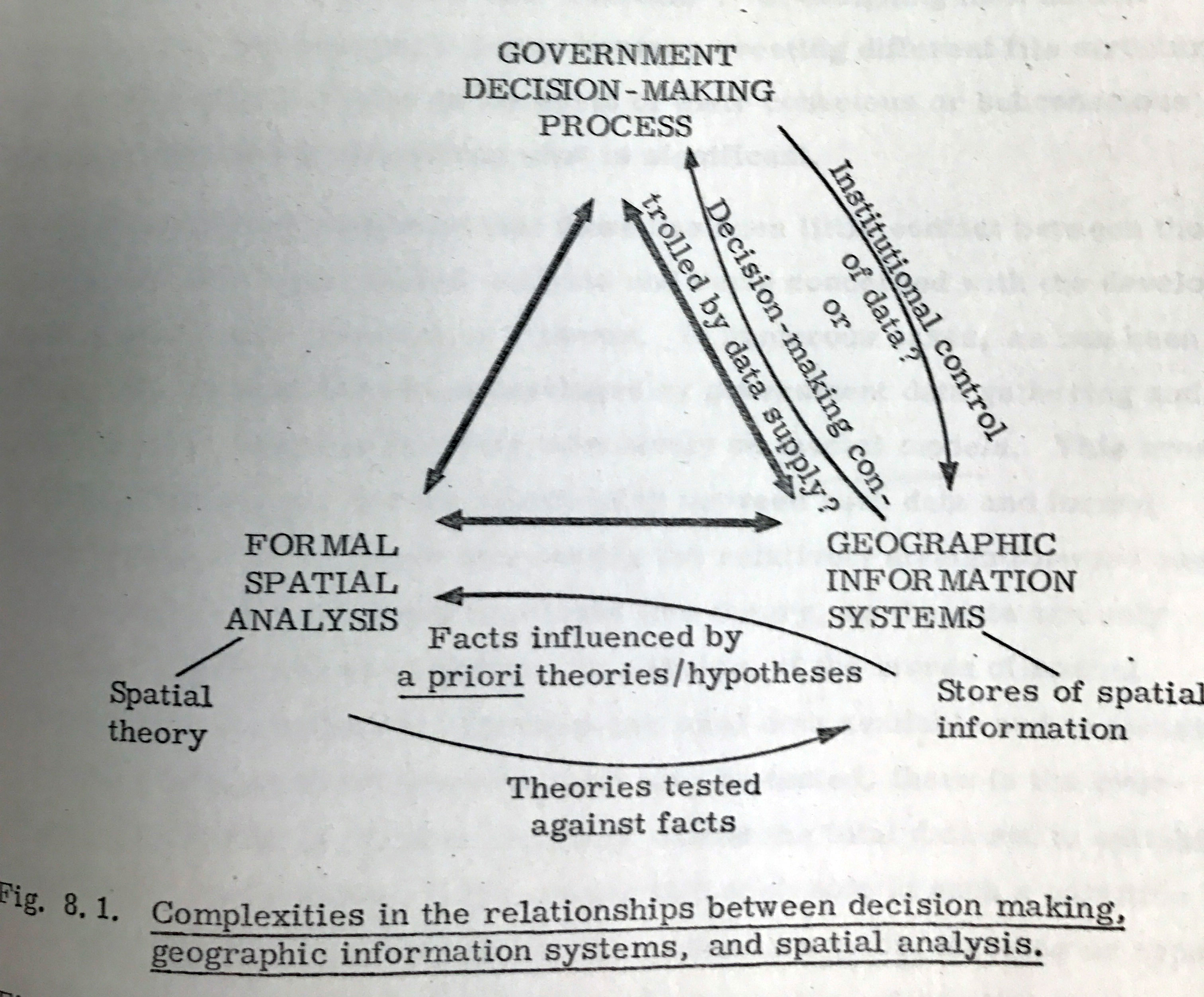
…but also in the governance and impact of geographic data in the real world.
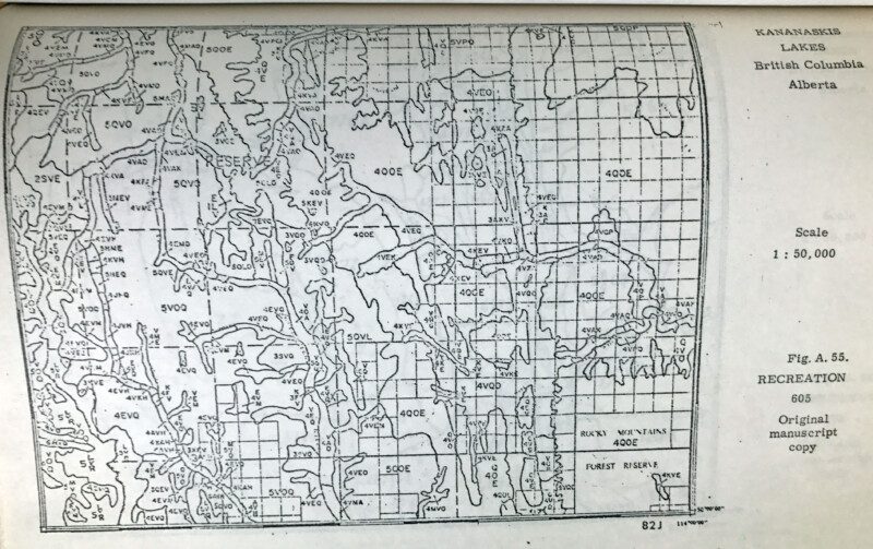
 The maps themselves are amongst the first to showcase the value of combining spatial data for insight – in this case for the identification of areas with high potential for particular land uses given a list of priorities.
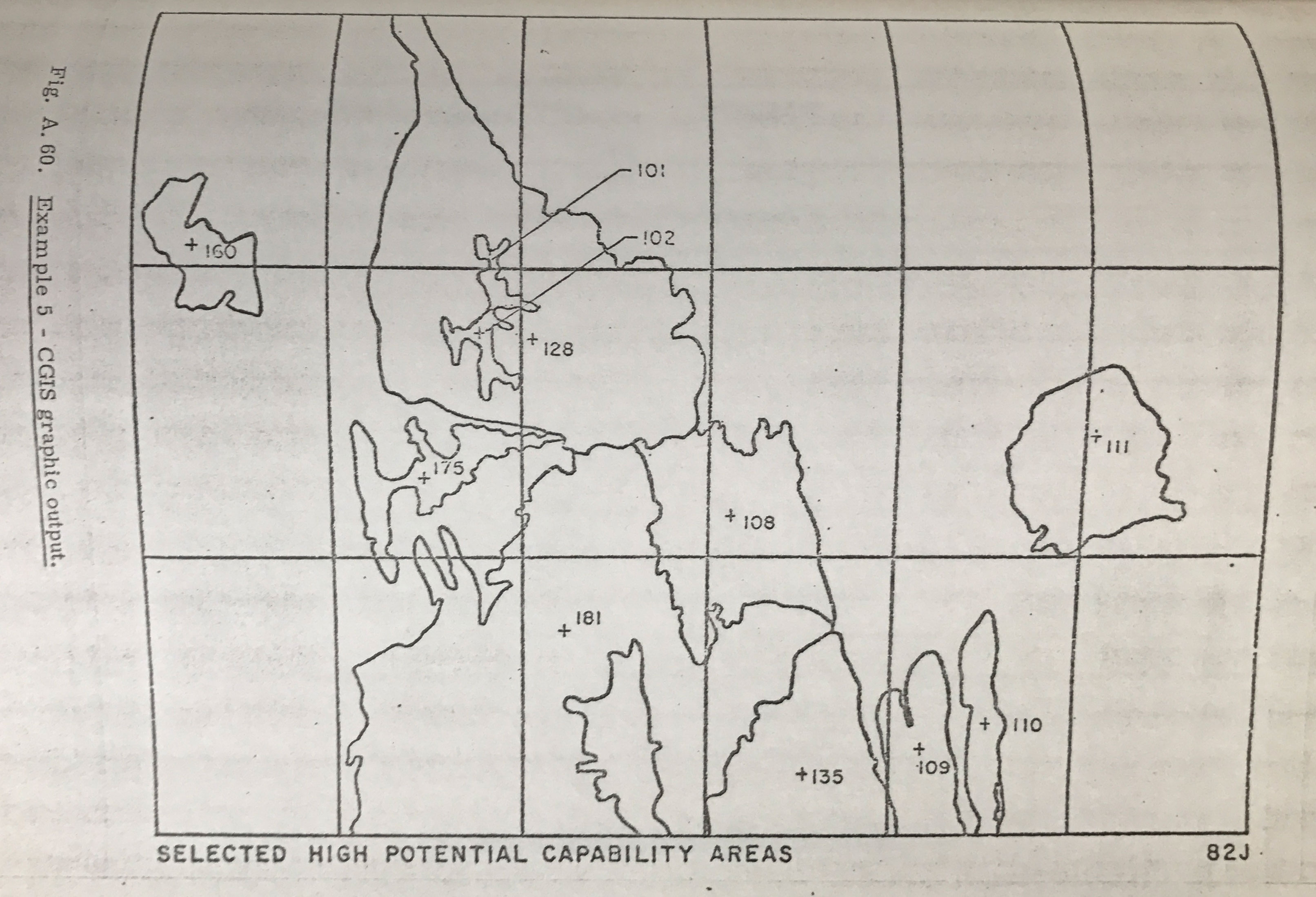
I was relieved to see that some things have changed since Tomlinson’s time as a PhD student. The thesis contains various tables of the costs – both in terms of person hours and $$ – for the various calculations required for his system. For example measuring the areas and perimeters of a few thousand polygons took 11.5 days (programming + processing) and cost $650 in CPU time!
Anyone working with spatial data should read this work at least once, if only because when we sought consent to post the work online Roger’s wife Lila said “I’m glad to hear that it will be disseminated far and wide”. Here’s the link again.

It has been a long held dream of mine to create a spinning globe using nothing but R (I wish I was joking, but I’m not). Thanks to the brilliant mapmate package created by Matt Leonawicz and shed loads of computing power, today that dream became a reality. The globe below took 19 hours and 30 processors to produce from a relatively low resolution NASA black marble data, and so I accept R is not the best software to be using for this – but it’s amazing that you can do this in R at all!

The code I used to do this is posted below. Under the hood the ggplot2 package is used for the plotting, so the first few data prep steps are taking the raster and converting it into a format that works with that. For information about installing the required packages and some other examples see the mapmate vignette here – there’s a lot more to it than the below. The black marble dataset is from here.
#Load in the packages
library(raster)
library(mapmate)
library(dplyr)
library(geosphere)
library(data.table)
library("parallel")
library(purrr)
library(RColorBrewer)
library(classInt)
#Load in the raster data
marble<-raster("BlackMarble_2016_3km_geo.tif")
#Simplify the raster - to test this out I would set the value at 50+
marble<- aggregate(marble, 10)
#Extact the values and coordinates from the raster grid - this is what is passed onto ggplot2.
marble.pts<-rasterToPoints(marble, spatial=T)
marble.pts@data <- data.frame(marble.pts@data, long=coordinates(marble.pts)[,1],lat=coordinates(marble.pts)[,2])
names(marble.pts@data)<- c("z","lon","lat")
#Convert to the tidyverse, required for mappmate.
marble.dat<-as_data_frame(marble.pts@data)
#We aren't plotting the image colours - rather a series of rectangles to be coloured by the pixel value. The range of colours needs to be specified. For this I have extraced the main colours from NASA's image and approximately aligned them to their corresponding values. This is seen the colour palette below that gets fed into the map.
pal<-colorRampPalette(c("#0b0c1a","#1e1c37","#202144","#2b3355","#7f6e61","#d0b695","#efd7af", "#fefbe6"), bias=2.75)
n<-30
#some more magic here - see the vignette I link to above.
marble.frame <- map(1:n, ~mutate(marble.dat, frameID = .x))
rng <- range(marble.dat$z, na.rm=TRUE)
file <- "3D_rotating_simp"
id<- "frameID"
#OK - here goes! You need the parallel package up and running - mc.cores specifies how many processors to use. You can see I used 30 but this can obviously be less.
mclapply(marble.frame, save_map,z.name="z", id=id, lon=0, lat=0, n.period=30, n.frames=n, col=pal(5000), type="maptiles", file=file, z.range=rng,png.args = list(width = 30,
        height = 30, res = 300, bg = "transparent", units="cm"),rotation.axis = 0,mc.cores=30)
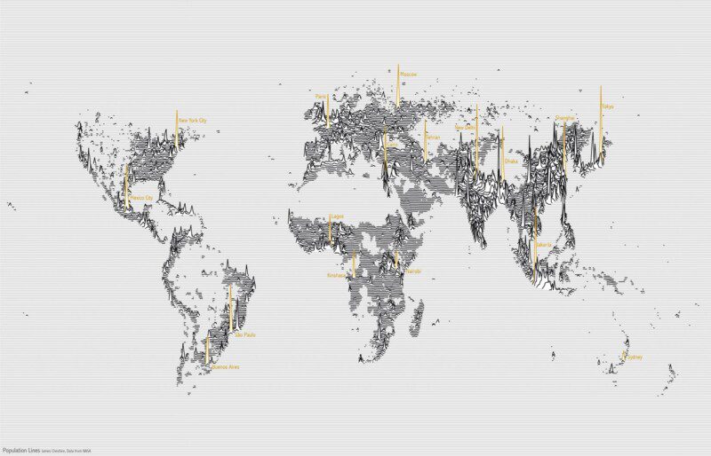
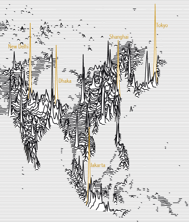
Thanks to the power of Reddit the “Population Lines” print (buy here) I created back in 2013 has attracted a huge amount of interest in the past week or so (a Europe only version made by Henrik Lindberg made the Reddit front page). There’s been lots of subsequent discussion about it’s inspiration, effectiveness as a form of visualisation and requests for the original code. So for the purposes of posterity I thought I’d run through the map’s conception and history.
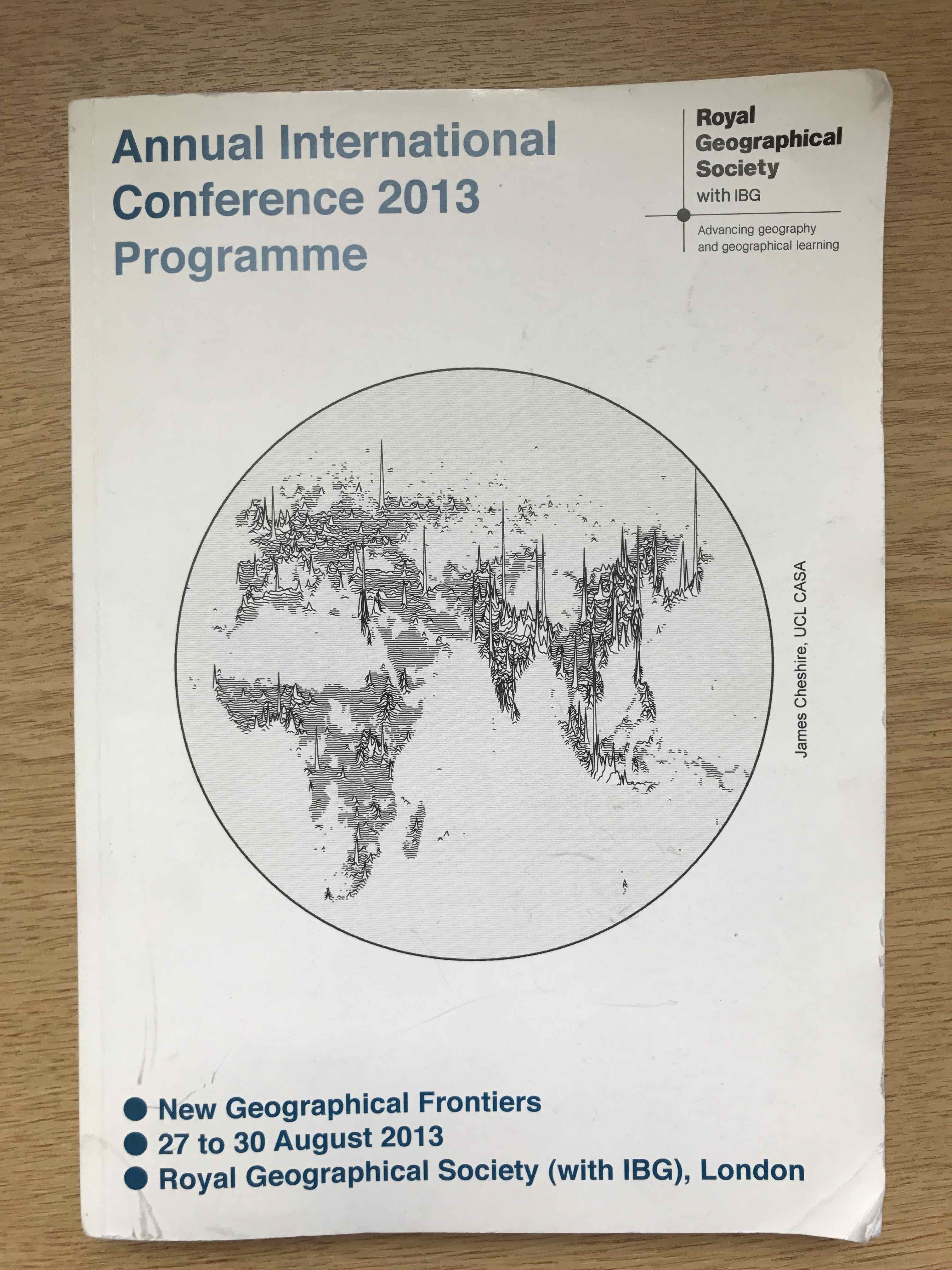
I was asked to create a graphic for the front cover for the programme of the Royal Geographical Society’s Annual Conference in 2013. The theme for the conference was “New Geographical Frontiers” and given the RGS’s long association with exploration I immediately thought of path breaking across undiscovered lands or summiting mountains. These activities have very little to do with the annual conference, but I wanted to evoke them a little on the cover. To me the greatest frontier for geographers is better understanding the world population and also appreciating that Europe/ the USA are no longer at the centre of the action. I therefore played around with various population map options (you can see some inspiration ideas here). I was keen to get something that showed the true peaks of global population, which is how I came upon what I thought was a fairly original idea of showing population density spikes along lines of latitude using data from NASA’s SEDAC. After creating this – and as with so many things in geography/cartography/ dataviz – I later discovered that mapping spatial data in this way had been done before by the pioneers of computer mapping using software called SYMAP (I can’t find an image of this but I’ve definitely seen it!). So it’s nothing new in terms of a way of geographically representing the world.
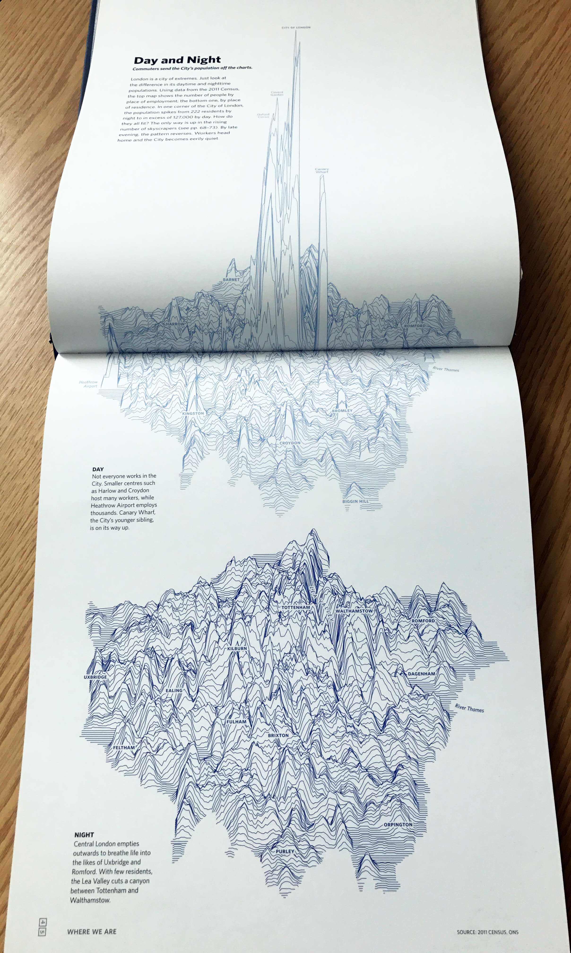
As for the design I was seeking something akin to the iconic Joy Division album cover. The original RGS cover was black and white, but thanks to a suggestion from Oliver, I opted to mark key cities in gold to help with orientation etc. I’ve provided the original R code below for those interested. Since creating Population Lines I’ve only created one other map using this technique and it was for the book London: the Information Capital. For this we wanted to show the huge population spike experienced but The City of London during the working day. I think it works really well for this. I’m not convinced the technique is good at showing exact data values at precise locations but if you are looking to draw attention to extremes and you are dealing with familiar geographies/ places then it can tell a compelling story.
 R Code
Here is the original R code I used back in May 2013. R has come on a lot since then, but this still works! You should use the latest population grid from NASA’s SEDAC.
#Load packages library(sp) library(rgdal) library(reshape) library(ggplot2) library(maptools) library(rgeos)#create a range standardisation function range01 <- function(x){(x-min(x))/(max(x)-min(x))} #load in a population grid - in this case it's population density from NASA's SEDAC (see link above). It's spatial data if you haven't seen this before in R. input<-readGDAL("glp10ag30.asc") # the latest data come as a Tiff so you will need to tweak.
## glp10ag30.asc has GDAL driver AAIGrid
## and has 286 rows and 720 columns
proj4string(input) = CRS("+init=epsg:4326")## Warning in `proj4string<-`(`*tmp*`, value = <S4 object of class structure("CRS", package = "sp")>): A new CRS was assigned to an object with an existing CRS:
## +proj=longlat +datum=WGS84 +no_defs +ellps=WGS84 +towgs84=0,0,0
## without reprojecting.
## For reprojection, use function spTransform#Get the data out of the spatial grid format using "melt" and rename the columns.
values<-melt(input)
names(values)<- c("pop", "x", "y")
#Rescale the values. This is to ensure that you can see the variation in the data
values$pop_st<-range01(values$pop)*0.20
values$x_st<-range01(values$x)
values$y_st<-range01(values$y)
#Switch off various ggplot things
xquiet<- scale_x_continuous("", breaks=NULL)
yquiet<-scale_y_continuous("", breaks=NULL)
quiet<-list(xquiet, yquiet)
#Add 180 to the latitude to remove negatives in southern hemisphere, then order them.
values$ord<-values$y+180
values_s<- values[order(-values$ord),]
#Create an empty plot called p
p<-ggplot()
#This loops through each line of latitude and produced a filled polygon that will mask out the lines beneath and then plots the paths on top.The p object becomes a big ggplot2 plot.
for (i in unique(values_s$ord))
{
p<-p+geom_polygon(data=values_s[values_s$ord==i,],aes(x_st, pop_st+y_st,group=y_st), size=0.2, fill="white", col="white")+ geom_path(data=values_s[values_s$ord==i,],aes(x_st, pop_st+y_st,group=y_st),size=0.2, lineend="round")
}
#show plot!
p +theme(panel.background = element_rect(fill='white',colour='white'))+quietIf you want to learn more, you can see here for another tutorial that takes a slightly different approach with the same effect.
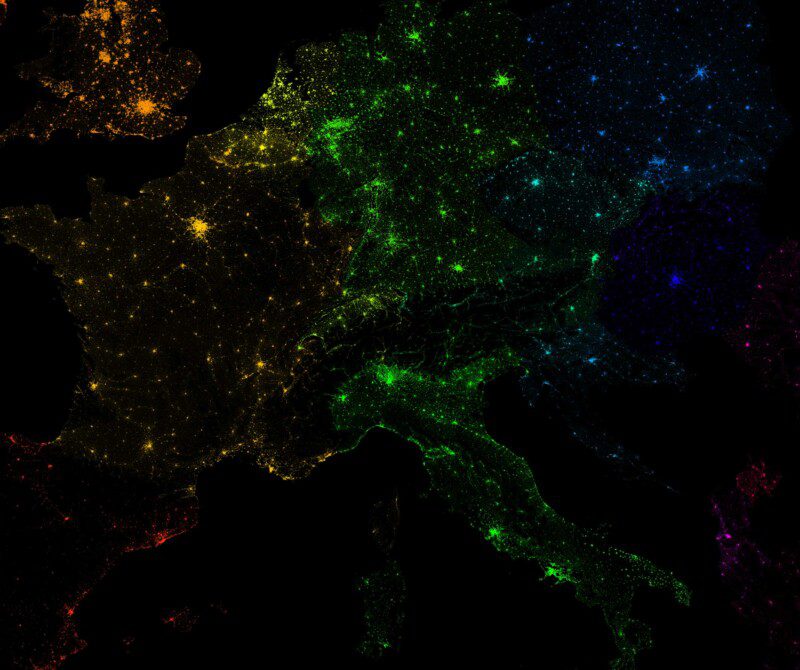
Dot density maps are an increasingly popular way of showing population datasets. The technique has its limitations (see here for more info), but it can create some really nice visual outputs, particularly when trying to show density. I have tried to push this to the limit by using a high resolution population grid for Europe (GEOSTAT 2011) to plot a dot for every 50 people in Europe (interactive). The detailed data aren’t published for all European countries – there are modelled values for those missing but I have decided to stick to only those countries with actual counts here.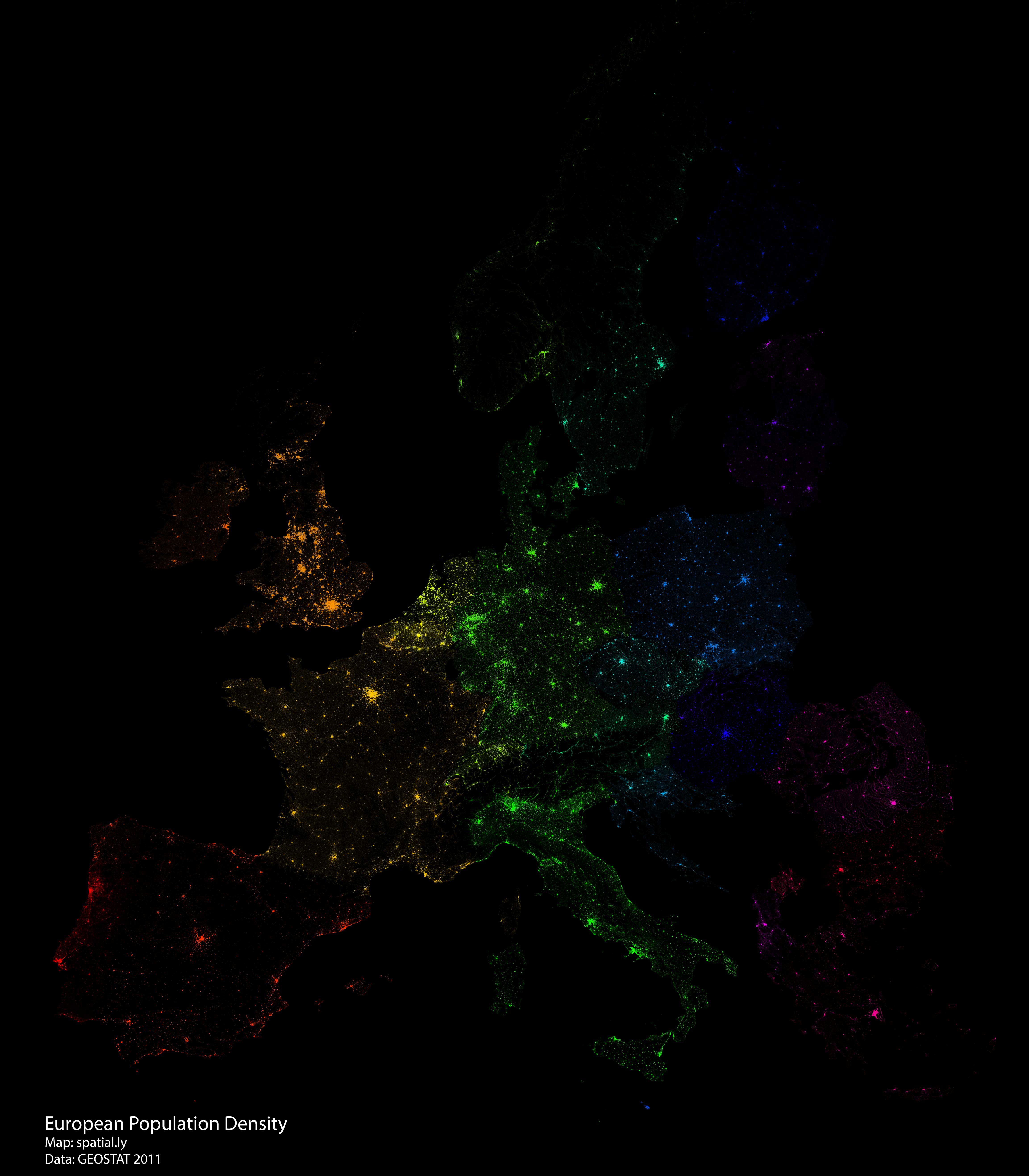
I produced this map as part of an experiment to see how R could handle generating millions of dots from spatial data and then plotting them. Even though the final image is 3.8 metres by 3.8 metres – this is as big as I could make it without causing R to crash – many of the grid cells in urban areas are saturated with dots so a lot of detail is lost in those areas. The technique is effective in areas that are more sparsely populated. It would probably work better with larger spatial units that aren’t necessarily grid cells.
Generating the dots (using the spsample function) and then plotting them in one go would require way more RAM than I have access to. Instead I wrote a loop to select each grid cell of population data, generate the requisite number of points and then plot them. This created a much lighter load as my computer happily chugged away for a few hours to produce the plot. I could have plotted a dot for each person (500 million+) but this would have completely saturated the map, so instead I opted for 1 dot for every 50 people.
I have provided full code below. T&Cs on the data mean I can’t share that directly but you can download here.
Load rgdal and the spatial object required. In this case it’s the GEOSTAT 2011 population grid. In addition I am using the rainbow function to generate a rainbow palette for each of the countries.
library(rgdal)
Input<-readOGR(dsn=".", layer="SHAPEFILE")
Cols<- data.frame(Country=unique(Input$Country), Cols=rainbow(nrow(data.frame(unique(Input$Country)))))
Create the initial plot. This is empty but it enables the dots to be added interatively to the plot. I have specified 380cm by 380cm at 150 dpi PNG – this is as big as I could get it without crashing R.
png("europe_density.png",width=380, height=380, units="cm", res=150)
par(bg='black')
plot(t(bbox(Input)), asp=T, axes=F, ann=F)
Loop through each of the individual spatial units – grid cells in this case – and plot the dots for each. The number of dots are specified in spsample as the grid cell’s population value/50.
for (j in 1:nrow(Cols))
{
Subset<- Input[Input$Country==Cols[j,1],]
for (i in 1:nrow(Subset@data))
  {
  Poly<- Subset[i,]
  pts1<-spsample(Poly, n = 1+round(Poly@data$Pop/50), "random", iter=15)
  #The colours are taken from the Cols object.
  plot(pts1, pch=16, cex=0.03, add=T, col=as.vector(Cols[j,2]))
  }
}
dev.off()
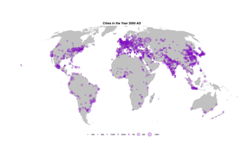
I recently stumbled upon a great dataset. It’s the first to provide comprehensive data for world city sizes as far back as 3700BC. The authors (Meredith Reba, Femke Reitsma & Karen Seto) write:
How were cities distributed globally in the past? How many people lived in these cities? How did cities influence their local and regional environments? In order to understand the current era of urbanization, we must understand long-term historical urbanization trends and patterns. However, to date there is no comprehensive record of spatially explicit, historic, city-level population data at the global scale. Here, we developed the first spatially explicit dataset of urban settlements from 3700 BC to AD 2000, by digitizing, transcribing, and geocoding historical, archaeological, and census-based urban population data previously published in tabular form by Chandler and Modelski.
These kinds of data are crying out to be mapped so that’s what I did…
I was keen to see how easy it was to produce an animated map with R and the ggplot2 package from these data. It turned out to be a slightly bigger job than I thought – partly because the cleaned data doesn’t have all the population estimates updating for every city each year so there’s a bit of a messy loop at the start of the code to get that bit working, and partly because there a LOADS of different parameters to tweak on ggplot to get the maps looking the way I like. The script below will generate a series of PNGs that can be strung together into an animation using a graphics package. To learn how to convert these into an animation see this excellent tutorial by Lena Groeger. I’m a big fan of what ggplot2 can do now and I hope, at the very least, the chunks of ggplot2 code below will provide a useful template for similar mapping projects.
Load the libraries we need
library("ggplot2")
library("ggthemes")
library("rworldmap")
library("classInt")
library("gridExtra")
library("grid")
library("cowplot")
load data – this is the processed file from http://www.nature.com/articles/sdata201634 I offer no guarantees about whether I ran the script correctly etc! I’d encourage you to take the data direct from the authors.
#City data
cities<- read.csv("alldata.csv")
#for some reason the coords were loaded as factors so I've created two new numeric fields here
cities$X<-as.numeric(as.vector(cities$Longitude))
cities$Y<-as.numeric(as.vector(cities$Latitude))
#World map base from rworldmap
world <- fortify(getMap(resolution="low"))
Take a look at the data
head(cities)Create the base map
base<- ggplot() + geom_map(data=world, map=world, aes(x=long,y=lat, map_id=id, group=group),fill="#CCCCCC") +theme_map()Now plot the cities on top – with circles scaled by city size. Here I am using the mollweide projection. This script loops through the data and checks for updates from one year to the next. It then plots the cities as proportional circles for each year and saves out an image for each 100 years of data. If you are just interested in the maps themselves and have your own point data then most of the below can be ignored.
Set the breaks for the size of the circles
size_breaks<-c(10000,50000,100000,500000,1000000,5000000,10000000)#Here I'm looping through the data each year to select the years required and comparing/ updating the values for each city.
count<-1
for (i in unique(cities$year))
{
if (count==1)
{
Data<-cities[which(cities$year==i),]
}else{
New_Data<-cities[which(cities$year==i),]
#replace old rows
Data2<-merge(Data, New_Data, by.x="X", by.y="X", all=T)
New_Vals<-Data2[!is.na(Data2$pop.y),c("City.y","X","Y.y","pop.y")]
names(New_Vals)<-c("City","X","Y","pop")
Old_Vals<-Data2[is.na(Data2$pop.y),c("City.x","X","Y.x","pop.x")]
names(Old_Vals)<-c("City","X","Y","pop")
Data<-rbind(New_Vals,Old_Vals)
Data<- aggregate(Data$pop, by=list(Data$City,Data$X, Data$Y), FUN="mean")
names(Data)<-c("City","X","Y","pop")
}
#This statement sorts out the BC/ AC in the title that we'll use for the plot.
if(i<0)
{
title <- paste0("Cities in the Year ",sqrt(i^2)," BC")
}else{
title <- paste0("Cities in the Year ",i," AD")
}
#There's lots going on here with the myriad of different ggplot2 parameters. I've broken each chunk up line by line to help make it a little clearer.
Map<-base+
geom_point(data=Data, aes(x=X, y=Y, size=pop), colour="#9933CC",alpha=0.3, pch=20)+
scale_size(breaks=size_breaks,range=c(2,14), limits=c(min(cities$pop), max(cities$pop)),labels=c("10K","50k","100K","500k","1M","5M","10M+"))+
coord_map("mollweide", ylim=c(-55,80),xlim=c(-180,180))+
theme(legend.position="bottom",legend.direction="horizontal",legend.justification="center",legend.title=element_blank(),plot.title = element_text(hjust = 0.5,face='bold',family = "Helvetica"))+ggtitle(title)+guides(size=guide_legend(nrow=1))
#I only want to plot map every 100 years
if(i%%100==0)
{
png(paste0("outputs/",i,"_moll.png"), width=30,height=20, units="cm", res=150)
print(Map)
dev.off()
}
count<-count+1
}Just to make things a little more interesting I wanted to try a plot of two hemispheres (covering most, but not all) of the globe. I’ve also added the key in between them. This depends on the plot_grid() functionality as well as a few extra steps you’ll spot that we didn’t need above.
count<-1
for (i in unique(cities$year))
{
if (count==1)
{
  Data<-cities[which(cities$year==i),]
}else{
  New_Data<-cities[which(cities$year==i),]
  #replace old rows
  Data2<-merge(Data, New_Data, by.x="X", by.y="X", all=T)
  New_Vals<-Data2[!is.na(Data2$pop.y),c("City.y","X","Y.y","pop.y")]
  names(New_Vals)<-c("City","X","Y","pop")
  Old_Vals<-Data2[is.na(Data2$pop.y),c("City.x","X","Y.x","pop.x")]
  names(Old_Vals)<-c("City","X","Y","pop")
  Data<-rbind(New_Vals,Old_Vals)
  Data<- aggregate(Data$pop, by=list(Data$City,Data$X, Data$Y), FUN="mean")
  names(Data)<-c("City","X","Y","pop")
}
#Create a map for each hemisphere - to help with the positioning I needed to use the `plot.margin` options in the `theme()` settings.
map1<-base+geom_point(data=Data, aes(x=X, y=Y, size=pop), colour="#9933CC",alpha=0.3, pch=20)+scale_size(breaks=size_breaks,range=c(2,16), limits=c(min(cities$pop), max(cities$pop)))+coord_map("ortho", orientation = c(10, 60, 0),ylim=c(-55,70))+ theme(legend.position="none",plot.margin = unit(c(0.5,0.5,-0.1,0.5), "cm"))
map2<- base+geom_point(data=Data, aes(x=X, y=Y, size=pop), colour="#9933CC",alpha=0.3, pch=20)+scale_size(breaks=size_breaks,range=c(2,16),limits=c(min(cities$pop), max(cities$pop)))+coord_map("ortho", orientation = c(10, -90, 0),ylim=c(-55,70))+ theme(legend.position="none", plot.margin = unit(c(0.5,0.5,0,0.5), "cm"))
#create dummy plot that we will use the legend from - basically I just want to create something that has a legend (they've been switched off for the maps above)
dummy<-ggplot()+geom_point(aes(1:7,1,size=size_breaks),colour="#9933CC", alpha=0.3, pch=20)+scale_size(breaks=size_breaks,range=c(2,16),labels=c("10K","50k","100K","500k","1M","5M","10M+"),limits=c(min(cities$pop), max(cities$pop)))+theme(legend.position="bottom",legend.direction="vertical",legend.title=element_blank())+guides(size=guide_legend(nrow=1,byrow=TRUE))
Legend <- get_legend(dummy)
#This statement sorts out the BC/ AC in the title.
if(i<0)
{
title <- ggdraw() + draw_label(paste0("Cities in the Year ",sqrt(i^2)," BC"), fontface='bold',fontfamily = "Helvetica")
}else{
  title <- ggdraw() + draw_label(paste0("Cities in the Year ",i," AD"), fontface='bold',fontfamily = "Helvetica")
}
#I only want to plot map every 100 years
if(i%%100==0)
{
png(paste0("outputs/",i,".png"), width=20,height=30, units="cm", res=150)
#This is where the elements of the plot are combined
print(plot_grid(title,map1, Legend,map2, ncol=1,rel_heights = c(.1,1, .1,1)))
dev.off()
}
count<-count+1
}
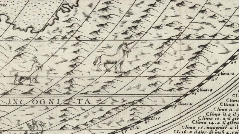
I recently had the pleasure of giving a Creative Mornings talk. Each month there is a new theme that the presenters need to refer to – mine was “fantasy” so I chose to open with one of my favourite fantasy creatures: the unicorn. It’s a talk about the creative process behind Oliver Uberti and I’s latest book Where the Animals Go. The talk touches on the value of picking out stories in big data and also how we should try to work together and play to our strengths. In short it’s about how we should to aspire to be less like elusive unicorns and more like cooperative and democratic baboons.